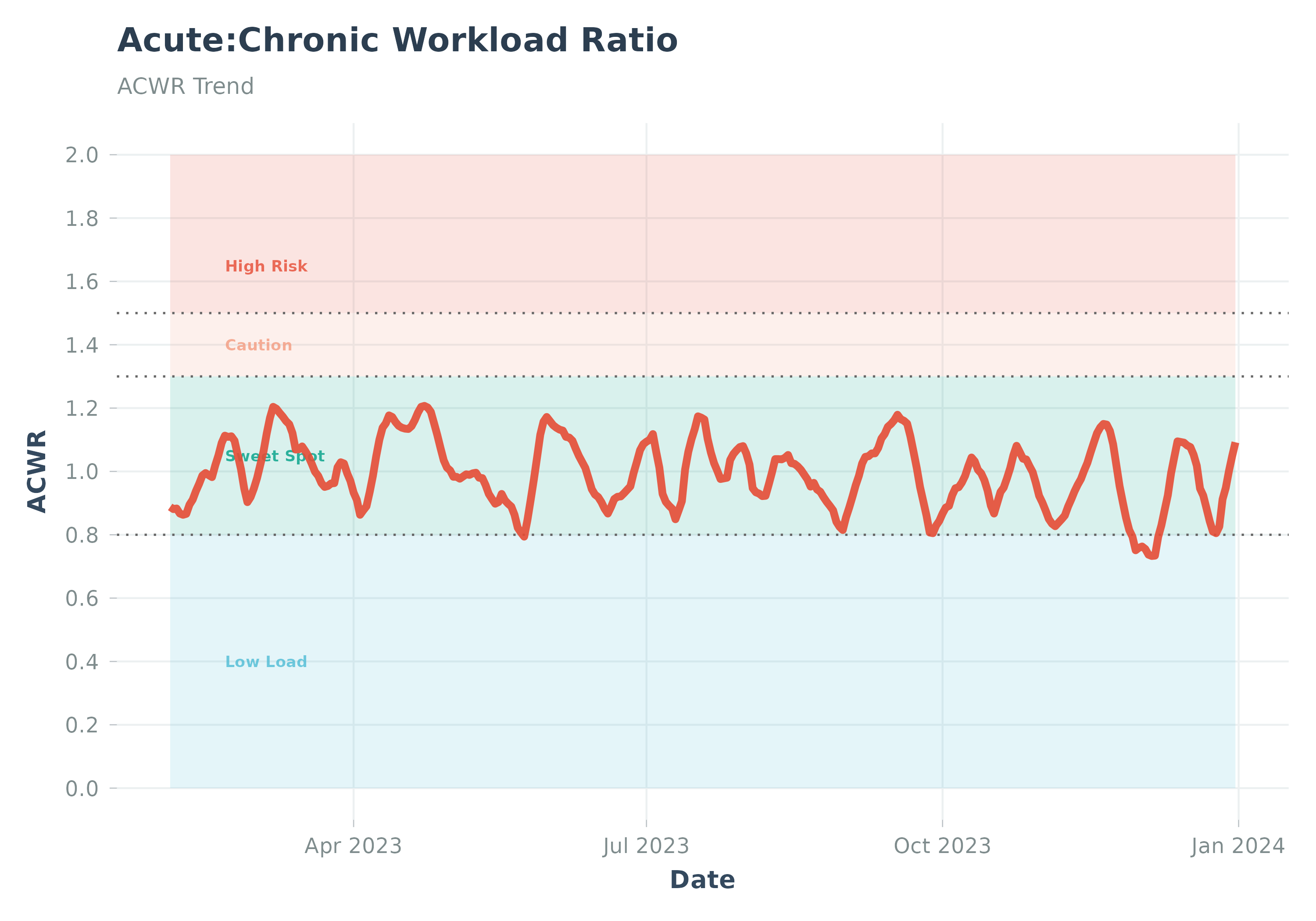
Visualizes the Acute:Chronic Workload Ratio (ACWR) trend over time.
Usage
plot_acwr(
  data,
  highlight_zones = TRUE,
  sweet_spot_min = 0.8,
  sweet_spot_max = 1.3,
  high_risk_min = 1.5,
  group_var = NULL,
  group_colors = NULL,
  title = NULL,
  subtitle = NULL,
  ...
)
Arguments
- data
A data frame from
calculate_acwr()orcalculate_acwr_ewma(). Must containdateandacwr_smoothcolumns.- highlight_zones
Logical, whether to highlight descriptive ACWR bands (e.g., reference band, high ACWR) on the plot. Default
TRUE.- sweet_spot_min
Lower bound for the reference ACWR band. Default 0.8.
- sweet_spot_max
Upper bound for the reference ACWR band. Default 1.3.
- high_risk_min
Lower bound for the high-ACWR band. Default 1.5.
- group_var
Optional. Column name for grouping/faceting (e.g., "athlete_id").
- group_colors
Optional. Named vector of colors for groups.
- title
Optional. Custom title for the plot.
- subtitle
Optional. Custom subtitle for the plot.
- ...
Additional arguments. Arguments
activity_type,load_metric,acute_period,chronic_period,start_date,end_date,user_ftp,user_max_hr,user_resting_hr,smoothing_period,acwr_dfare deprecated and ignored.
Details
Plots the ACWR trend over time.
Best practice: Use calculate_acwr() first, then pass the result to this function.
ACWR is calculated as acute load / chronic load. The default 0.8-1.3
band is a commonly used reference band.
When highlight_zones = TRUE, all zone labels (High ACWR, Elevated ACWR,
Reference Band, Low ACWR) are always displayed regardless of whether
data falls within each zone.
The y-axis is automatically extended to ensure all zone annotations remain visible.
Zone boundaries can be customised via sweet_spot_min, sweet_spot_max, and
high_risk_min.
Note: The predictive value of ACWR for injury outcomes is debated in the
literature (Impellizzeri et al., 2020). Zone labels should be interpreted
as descriptive workload heuristics, not validated injury predictors. See
calculate_acwr() documentation for full references.