Reads raw audio data from any common audio or video format. Use read_audio_bin to get raw PCM audio samples, or read_audio_fft to stream-convert directly into frequency domain (spectrum) data using FFmpeg built-in FFT.
Usage
read_audio_fft(
  audio,
  window = hanning(1024),
  overlap = 0.75,
  sample_rate = NULL,
  start_time = NULL,
  end_time = NULL
)

read_audio_bin(
  audio,
  channels = NULL,
  sample_rate = NULL,
  start_time = NULL,
  end_time = NULL
)

write_audio_bin(
  pcm_data,
  pcm_channels = 1L,
  pcm_format = "s32le",
  output = "output.mp3",
  ...
)
Arguments
- audio
path to the input sound or video file containing the audio stream
- window
vector with weights defining the moving fft window function. The length of this vector is the size of the window and hence determines the output frequency range.
- overlap
value between 0 and 1 of overlap proportion between moving fft windows
- sample_rate
downsample audio to reduce FFT output size. Default keeps sample rate from the input file.
- start_time, end_time
position (in seconds) to cut input stream to be processed.
- channels
number of output channels, set to 1 to convert to mono sound
- pcm_data
integer vector as returned by read_audio_bin
- pcm_channels
number of channels in the data. Use the same value as you entered in read_audio_bin.
- pcm_format
this is always
s32le(signed 32-bit integer) for now- output
passed to av_audio_convert
- ...
other paramters for av_audio_convert
Details
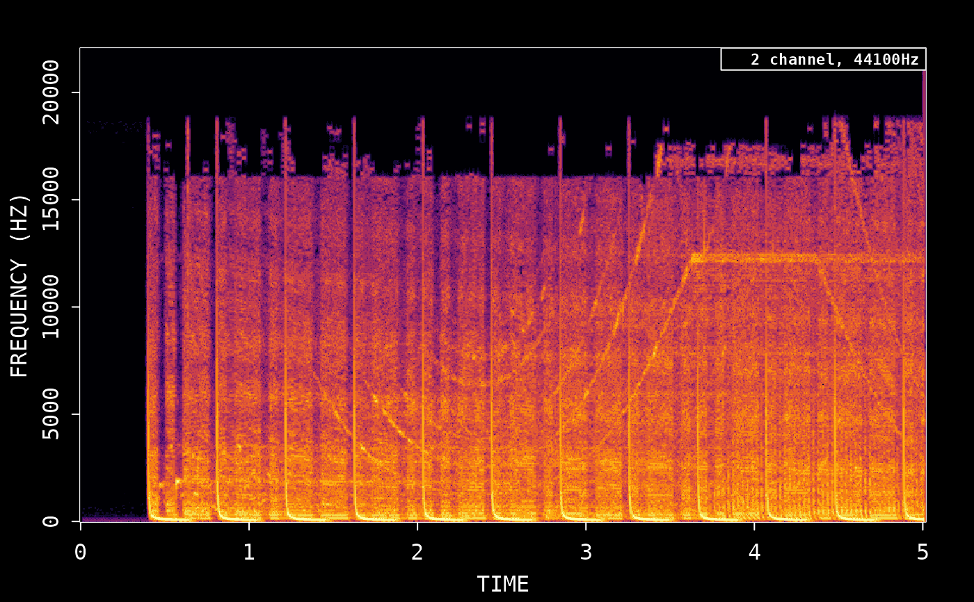
Currently read_audio_fft automatically converts input audio to mono channel such
that we get a single matrix. Use the plot() method on data returned by read_audio_fft
to show the spectrogram. The av_spectrogram_video generates a video that plays
the audio while showing an animated spectrogram with moving status bar, which is
very cool.
Examples
# Use a 5 sec fragment
wonderland <- system.file('samples/Synapsis-Wonderland.mp3', package='av')

# Read initial 5 sec as as frequency spectrum
fft_data <- read_audio_fft(wonderland, end_time = 5.0)
dim(fft_data)
#> [1] 512 860

# Plot the spectrogram
plot(fft_data)


# Show other parameters
dim(read_audio_fft(wonderland, end_time = 5.0, hamming(2048)))
#> [1] 1024  430
dim(read_audio_fft(wonderland, end_time = 5.0, hamming(4096)))
#> [1] 2048  215
# Show other parameters
dim(read_audio_fft(wonderland, end_time = 5.0, hamming(2048)))
#> [1] 1024 430
dim(read_audio_fft(wonderland, end_time = 5.0, hamming(4096)))
#> [1] 2048 215