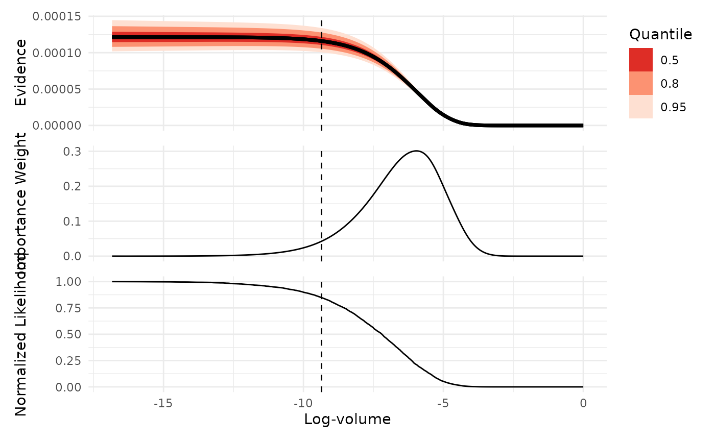
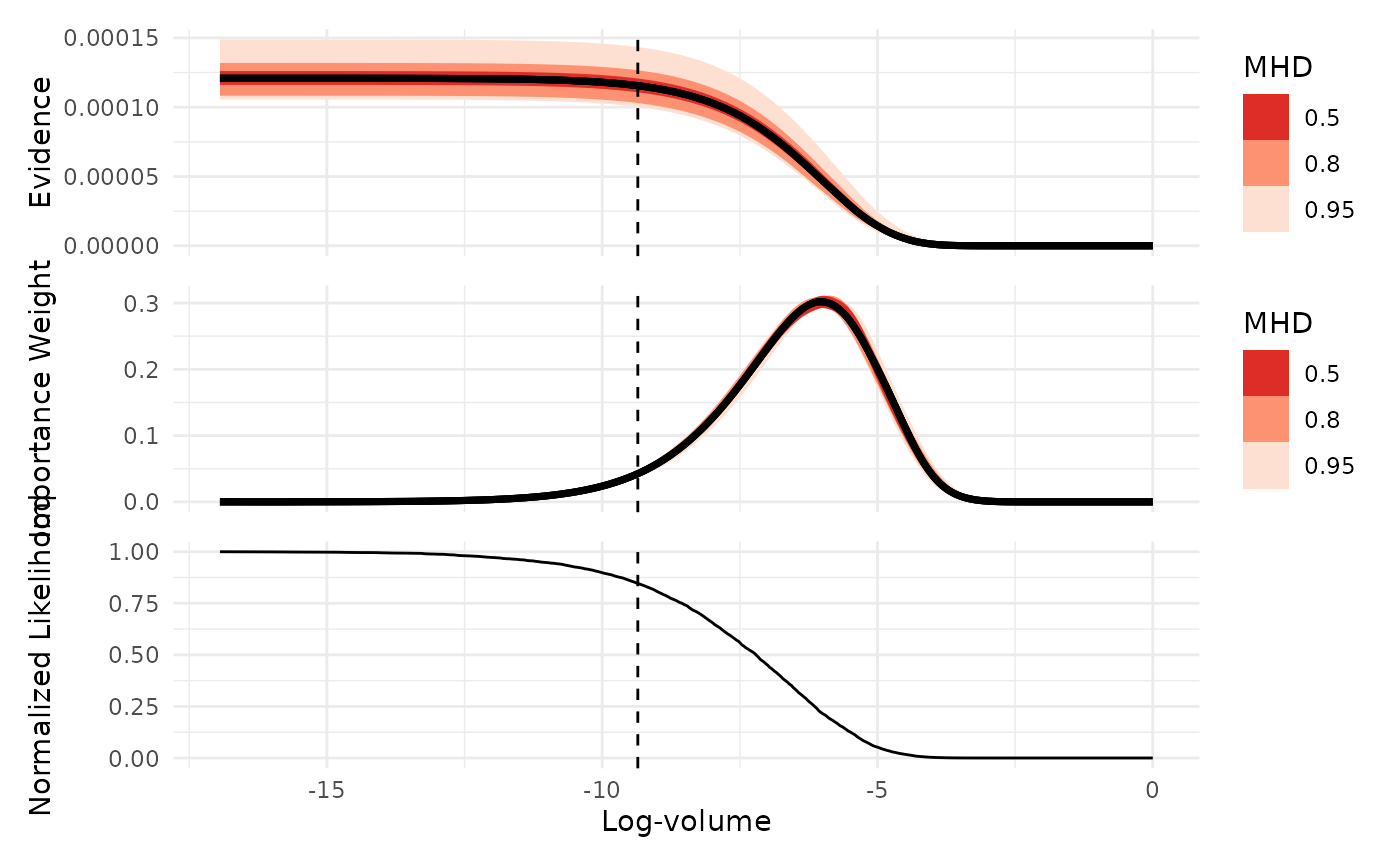
Visualizes key diagnostics from nested sampling outputs as functions of log-prior volume.
Usage
# S3 method for class 'ernest_estimate'
plot(x, which = c("evidence", "weight", "likelihood"), n = 512, ...)

# S3 method for class 'ernest_run'
plot(x, which = c("evidence", "weight", "likelihood"), n = 512, ...)

# S3 method for class 'ernest_estimate'
summary(
  object,
  which = c("evidence", "weight", "likelihood"),
  n = 512,
  width = NULL,
  ...
)
Arguments
- x, object
[ernest_run] or [ernest_estimate]
An object containing results from nested sampling.- which
[character()]
One or more diagnostics to display. Must be any of"evidence","weight", and"likelihood".- n
[integer(1)]
Number of evaluation points along the log-volume axis used to summarize each curve.- ...
These dots are for future extensions and must be empty.
- width
[numeric()]
Numeric vector of widths for uncertainty intervals. Defaults to the 50%, 80%, and 95% highest mean depth intervals.
Value
For plot, the ggplot object, invisibly. It is also printed as a side
effect.
For summary, a list with possible elements evidence, weight,
and likelihood. Each element is a data frame.
Details
plot() is a visualization wrapper around summary.ernest_estimate(),
followed by autoplot(). Use which to select diagnostics:
which = "evidence": Estimated marginal likelihood as a function of log-prior volume.which = "weight": Posterior mass concentration across log-prior volume.which = "likelihood": Normalized likelihood across log-prior volume.
If x is an ernest_run, plotting first computes
calculate(x, ndraws = 0). In this mode, log_volume and log_weight are
deterministic, and evidence uncertainty comes from the analytical normal
approximation generated from the original sampling run.
If x is an ernest_estimate generated with ndraws > 0, diagnostics are
summarized over simulated log-volume trajectories. For these simulated
estimates, uncertainty bands for evidence and weight are computed as
interval summaries on interpolated curves.
To get the underlying data frames used for plotting, use
summary.ernest_estimate(). This is useful when you want full control over
plotting.
Note
Plotting multiple diagnostics with which requires patchwork.
Plotting evidence or weight diagnostics requires ggdist.
See also
Other visualizations:
visualize.ernest_run()