Extending the INTERGROWTH-21st Newborn Size Standards
Source:vignettes/articles/extending-ig-nbs.rmd
extending-ig-nbs.rmdRationale
Over the years, there have been many requests from users of the INTERGROWTH-21st Newborn Size Standards (including the Very Preterm standards) to extend their range from 168 to 300 days (24+0 to 42+6 weeks) gestational age (GA) to a wider span of 154 to 314 days (22+0 to 44+6 weeks) GA. We’ve decided to implement this in gigs as an entirely separate standard from the INTERGROWTH-21st Newborn Size standards, to make these extended versions of the standards available to all.
We want to note here that this process has been checked over by the former Lead Statistician for the INTERGROWTH-21st Project, Eric Ohuma, but is not endorsed officially by INTERGROWTH-21st. We want users to be aware that z-scores/centiles derived from these extended bounds must be used with caution - it is at the user’s discretion to ensure they are careful with these extended standards.
Approach
For the Very Preterm standards
For the INTERGROWTH-21st Very Preterm standards, extending the standards is easy. The Very Preterm standards use simple equations to model the mean and standard deviation at different gestational ages (GAs). Extending these standards is as simple as using gestational age values from 154 to 167 in these equations.
For the Newborn Size standards
The INTERGROWTH-21st Newborn Size standards are more
difficult to extend as they are coefficient-based. For each gestational
age from 231 days (33+0 weeks) to 300 days (42+6
weeks), there are corresponding mu/sigma/nu/tau values. These are used
with gamlss.dist::pST3() to convert values to centiles in
these standards, and with gamlss.dist::qST3() to convert
centiles to values. Each coefficient represents a different aspect of
the distribution of anthropometric measures at a given gestational
age:
-
mu- The median of the distribution at a given GA. -
sigma- The standard deviation of the distribution at a given GA. -
nu- The skewness of the distribution at a given GA. -
tau- The kurtosis of the distribution at a given GA.
To extend these standards out, we need to generate new coefficients
for gestational ages from 301 to 314 days (43+0 to
44+6 weeks). We will do this with fractional polynomial
regression in {mfp} package.
Extrapolating coefficients for the Newborn Size Standards
The mu and sigma values are different
across GAs for each standard. Luckily, the nu and
tau parameters are identical across all gestational ages
for most of these standards. Using unique(), we see that
for all INTERGROWTH-21st Newborn Size standards except female
length-for-GA (lfga/female), nu
and tau are constant.
#> Weight-for-GA:
#>  Male:
#>       Unique `nu` values: 1.095261
#>       Unique `tau` values: 17.05299
#>  Female:
#>       Unique `nu` values: 1.126787
#>       Unique `tau` values: 19.65738
#>
#> Length-for-GA:
#>  Male:
#>       Unique `nu` values: 1.007603
#>       Unique `tau` values: 15.4146
#>  Female:
#>       Unique `nu` values: 0.967756, 0.9677558
#>       Unique `tau` values: 19.95849
#>
#> Head circumference-for-GA:
#>  Male:
#>       Unique `nu` values: 1.033177
#>       Unique `tau` values: 26.17975
#>  Female:
#>       Unique `nu` values: 1.045915
#>       Unique `tau` values: 20.97268
Looking at the nu values for length-for-GA in females,
we see that only the first value is different (0.9677560).
Every other value in this vector is 0.9677568:
gigs::ig_nbs_coeffs$lfga$female$nu#> [1] 0.9677560 0.9677558 0.9677558 0.9677558 0.9677558 0.9677558 0.9677558
#> [8] 0.9677558 0.9677558 0.9677558 0.9677558 0.9677558 0.9677558 0.9677558
#> [15] 0.9677558 0.9677558 0.9677558 0.9677558 0.9677558 0.9677558 0.9677558
#> [22] 0.9677558 0.9677558 0.9677558 0.9677558 0.9677558 0.9677558 0.9677558
#> [29] 0.9677558 0.9677558 0.9677558 0.9677558 0.9677558 0.9677558 0.9677558
#> [36] 0.9677558 0.9677558 0.9677558 0.9677558 0.9677558 0.9677558 0.9677558
#> [43] 0.9677558 0.9677558 0.9677558 0.9677558 0.9677558 0.9677558 0.9677558
#> [50] 0.9677558 0.9677558 0.9677558 0.9677558 0.9677558 0.9677558 0.9677558
#> [57] 0.9677558 0.9677558 0.9677558 0.9677558 0.9677558 0.9677558 0.9677558
#> [64] 0.9677558 0.9677558 0.9677558 0.9677558 0.9677558 0.9677558 0.9677558We will assume for this set of coefficients that nu is
equal to 0.967758 after 300 days’ GA; for all other sets of
coefficients we know that nu and tau are
constant throughout.
The mu and sigma parameters for each
standard require extrapolation. The following function uses
mfp::mfp() to model the slope of mu and
sigma values against GA in each set of standards using
fractional polynomials. The resulting fractional polynomial produced by
can then be used with predict() to extrapolate the slopes
out to 314 days’ GA.
extrapolate_msnt <- function(acronym, sex) {
  existing_coeffs <- gigs::ig_nbs_coeffs[[acronym]][[sex]]

  # Increase alpha cut-off from 0.05 to make `mfp()` 'take' to some standards
  alpha <- 0.15
  # Subset for fracpoly regresion; improves transition to >300 days vs. using
  # entire GA range
  modelling_cutoff <- 280
  modelling_coeffs <- dplyr::filter(existing_coeffs, gest_days >= modelling_cutoff)

  mfp_mu <- mfp::mfp(mu ~ fp(gest_days, df = 4), data = modelling_coeffs,
                     maxits = 200, alpha = alpha)

  coeffs_ext <- data.frame(gest_days = 231:314)
  coeffs_ext$mu <- predict(mfp_mu, newdata = coeffs_ext)

  mfp_sigma <- mfp::mfp(sigma ~ fp(gest_days, df = 4), data = modelling_coeffs,
                        maxits = 200, alpha = alpha)
  coeffs_ext$sigma <- predict(mfp_sigma, newdata = coeffs_ext)

  coeffs_ext$nu <- existing_coeffs$nu[2]
  coeffs_ext$tau <- existing_coeffs$tau[2]

  # Replace predicted coeffs with old coeffs for old GA range
  coeffs_ext$mu[seq_along(231:300)] <- existing_coeffs$mu
  coeffs_ext$sigma[seq_along(231:300)] <- existing_coeffs$sigma
  coeffs_ext
}
Let’s iterate through our different standards and sexes. We store the
results in ig_nbs_ext_coeffs:
ig_nbs_ext_coeffs <- list(wfga = list(male = NULL, female = NULL),
                          lfga = list(male = NULL, female = NULL),
                          hcfga = list(male = NULL, female = NULL))

for (acronym in c("wfga", "lfga", "hcfga")) {
  for (sex in c("male", "female")) {
    ig_nbs_ext_coeffs[[acronym]][[sex]] <- extrapolate_msnt(acronym, sex)
  }
}
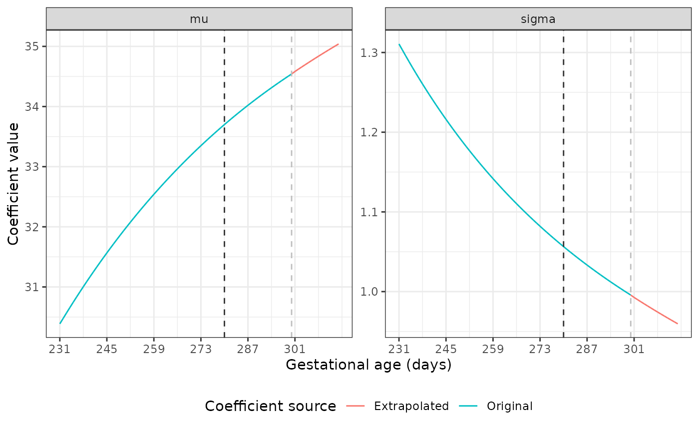
Plotting the extrapolated coefficients
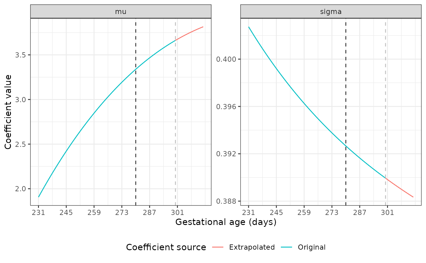
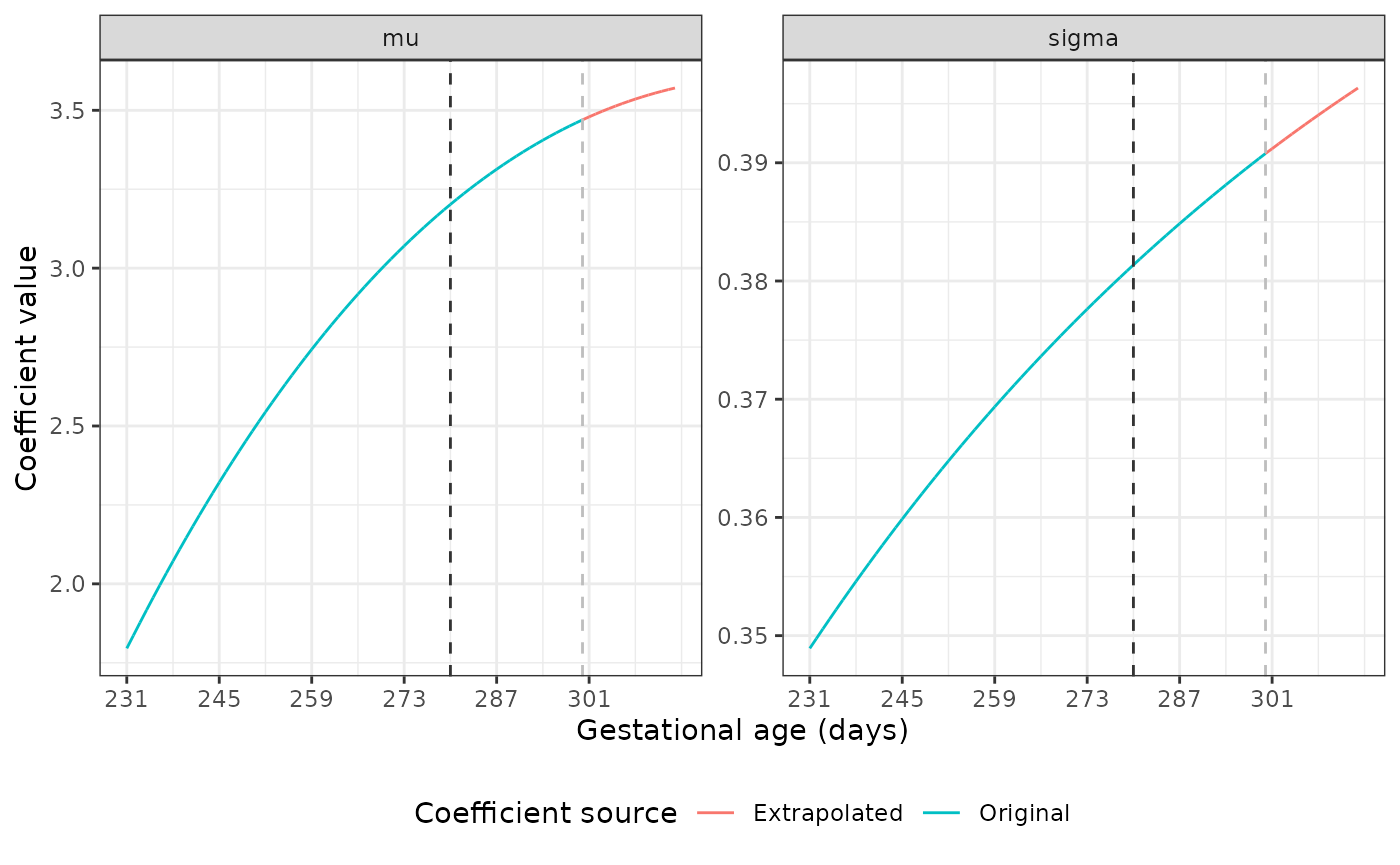
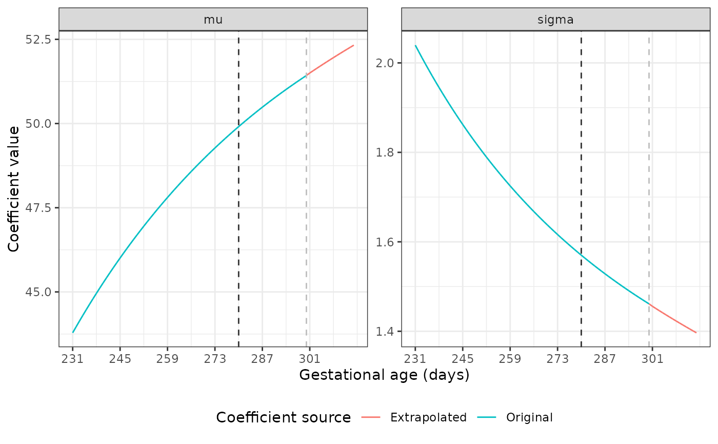
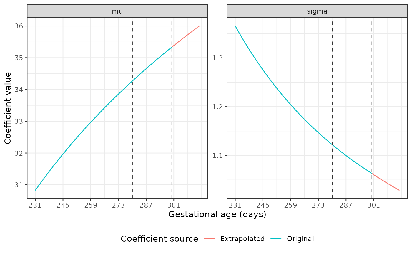
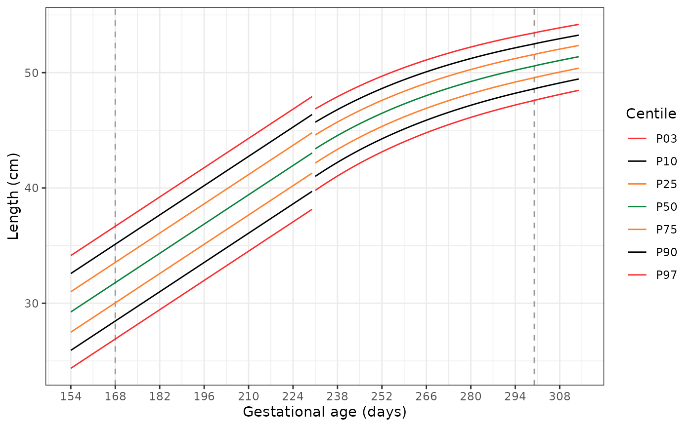
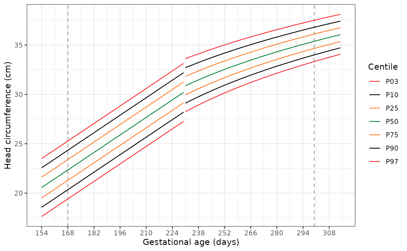
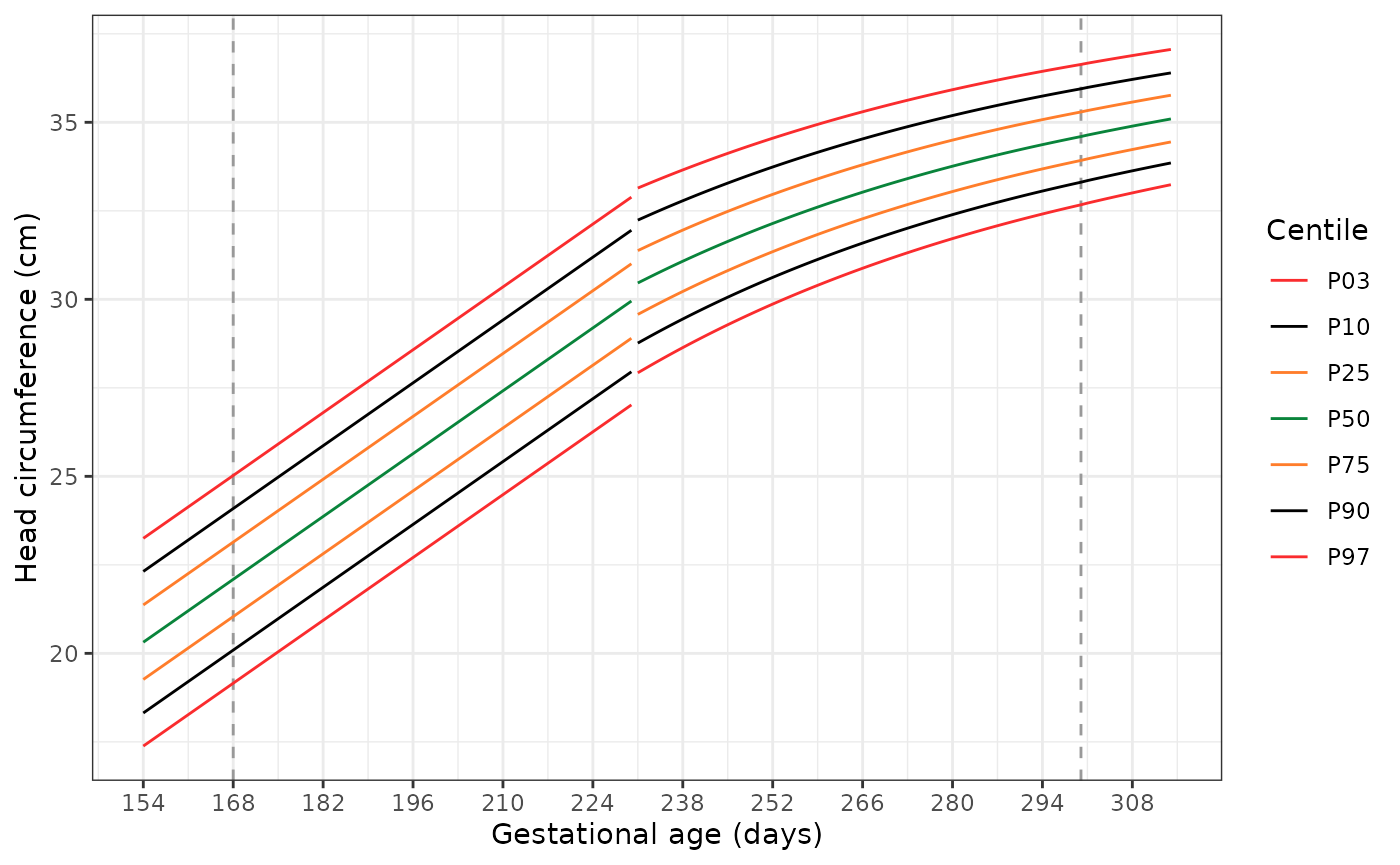
The dark grey dashed line marks the point at which we start using the original coefficient values to fit a fractional polynomial to the data. The light grey line shows where the extrapolation begins. Our plots show good extrapolations in these coefficients.
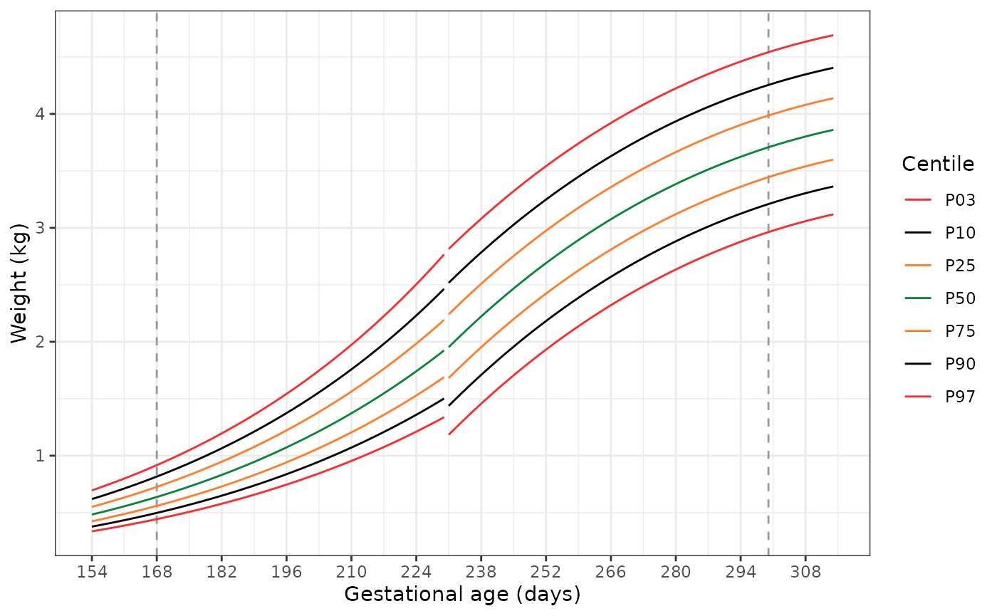
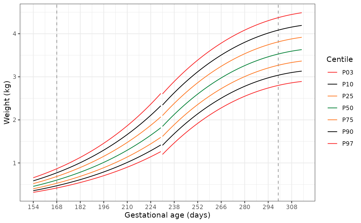
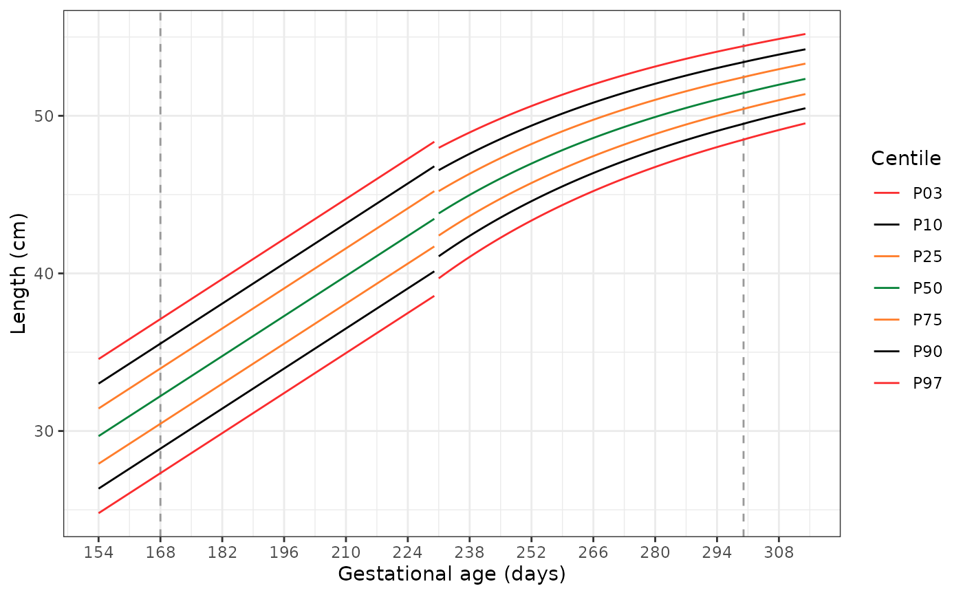
Plotting the extended standards
The following code has two functions. The first,
generate_extrapolated_ig_nbs(), produces a long data frame
with anthropometry for the 3rd, 10th,
25th, 50th, 75th, 90th, and
97th centiles. The second function
(plot_extrapolated_ig_nbs()) uses these to graph the
centiles, with grey dashed lines at 168 and 300 days to indicate where
extrapolation of the INTERGROWTH-21st Very Preterm Newborn
standards stops and extrapolation of the extrapolation of the
INTERGROWTH-21st Newborn Size standards starts, respectively.
Each plot has a gap at 231 days (33+0 weeks), where we switch
from using the INTERGROWTH-21st Very Preterm standards to the
INTERGROWTH-21st Newborn Size standards.
generate_extrapolated_ig_nbs <- function(acronym, sex) {
  purrr::map2(
    .x = c(0.03, 0.1, 0.25, 0.5, 0.75, 0.9, 0.97),
    .y = c("P03", "P10", "P25", "P50", "P75", "P90", "P97"),
    .f = function(centile, name) {
      vpns_lim <- 231
      gest_days <- 154:314
      y_nbs_ext <- with(ig_nbs_ext_coeffs[[acronym]][[sex]],
                        gamlss.dist::qST3C(p = centile,
                                            mu = mu,
                                            sigma = sigma,
                                            nu = nu,
                                            tau = tau))
      y_vpns_ext <- gigs:::ig_vpns_zscore2value(z = qnorm(centile),
                                                154:230,
                                                switch(sex,
                                                       male = "M",
                                                       female = "F"),
                                                acronym)
      standard <- ifelse(
        test = gest_days >= vpns_lim,
        yes = "NS",
        no = "Very Preterm NS"
      )
      x <- data.frame(gest_days = gest_days,
                      Centile = name,
                      y = c(y_vpns_ext, y_nbs_ext),
                      standard = standard)
    }) |>
    purrr::list_rbind()
}

plot_extrapolated_chart <- function(curve_data, acronym, sex) {
  key_colours <- c("P03" = "#fa2c2e",
                   "P10" = "black",
                   "P25" = "#ff7d2b",
                   "P50" = "#09843b",
                   "P75" = "#ff7d2b",
                   "P90" = "black",
                   "P97" = "#fa2c2e")
  ggplot2::ggplot(
    curve_data, ggplot2::aes(x = gest_days, y = y, colour = Centile,
                             id = standard)) +
    ggplot2::geom_vline(xintercept = 168, colour = "grey60", linetype = "dashed") +
    ggplot2::geom_vline(xintercept = 300, colour = "grey60", linetype = "dashed") +
    ggplot2::geom_line() +
    ggplot2::scale_x_continuous(breaks = seq(154, 314, 14),
                                labels = seq(154, 314, 14)) +
    ggplot2::scale_colour_manual(values = key_colours) +
    ggplot2::labs(
      x = "Gestational age (days)",
      y = switch(acronym,
                 "wfga" = "Weight (kg)",
                 "lfga" = "Length (cm)",
                 "hcfga" = "Head circumference (cm)"))
}Conclusion
In all, these extrapolated versions of the Newborn Size standards (incl. Very Preterm Newborns) should be useful for researchers with large datasets that contain relatively extreme gestational ages. Anyone utilising these extended standards in their work should do so with care, and note specifically that they used the extended versions.
