INTERGROWTH-21st Body Composition Equations

Though Villar et al. (2017) published centiles for body composition (fat mass, body fat percentage, and fat-free mass) in newborns from the INTERGROWTH-21^st project, they did not publish the parameters of the models used to generate their centiles. To implement these standards in gigs, we re-derived these values, in this case using the published data to work back to linear equations.

Contextual clues

To identify the way in which these body composition standards were modelled, we need to look into how the published centile tables are formatted. Consider the standard for fat mass for gestational age ("fmfga") in females:

fmfga_female

#> # A tibble: 5 × 6
#>   gest_days   P03   P10   P50   P90   P97
#>       <int> <int> <int> <int> <int> <int>
#> 1       266    29   123   324   525   619
#> 2       273    62   156   357   558   652
#> 3       280    96   190   391   592   686
#> 4       287   127   221   422   623   717
#> 5       294   150   244   445   646   740

Differences between each GA in fmfga

Let’s first compare the differences over time in fat-mass for GA. In each column, we’ll subtract the value of the previous row from the current row to produce a table of differences (see check_differences() below). Then we’ll check that the differences in each row are equal for all centiles, and store this in the all_equal column.

check_differences <- function(centile_tbl) {
  centile_tbl |>
    dplyr::mutate(dplyr::across(.cols = tidyselect::starts_with(match = "P"),
                                .fns = list(diff = \(x) x - dplyr::lag(x))),
                  .keep = "unused") |>
    dplyr::filter(dplyr::if_any(
            tidyselect::starts_with(match = "P"), ~ !is.na(.))) |>
    dplyr::rowwise() |>
    dplyr::mutate(
      all_equal = dplyr::n_distinct(P03_diff, P10_diff, P50_diff, P90_diff,
                                    P97_diff, na.rm = TRUE),
      all_equal = as.logical(all_equal)) |>
    dplyr::ungroup()
}

Let’s check the results for fmfga_female:

check_differences(fmfga_female)

#> # A tibble: 4 × 7
#>   gest_days P03_diff P10_diff P50_diff P90_diff P97_diff all_equal
#>       <int>    <int>    <int>    <int>    <int>    <int> <lgl>    
#> 1       273       33       33       33       33       33 TRUE     
#> 2       280       34       34       34       34       34 TRUE     
#> 3       287       31       31       31       31       31 TRUE     
#> 4       294       23       23       23       23       23 TRUE

The differences in fat mass are equal across percentiles at all gestational ages, according to the all_equal column. If the standard deviation ($\sigma$) changed with gestational age (GA), then all_equal would not be at each age. This hints that for these centile curves, the mean value ($\mu$) for fat mass was calculated first, then summed with the product of the desired $z$-score/centile with a standard deviation ($\sigma$) which is constant across the different GAs: $$\begin{align*} y = \mu + z\times\sigma \end{align*}$$

In the other standards

Does this equality hold for the other centile tables?

other_standards <- list(fmfga_male, bfpfga_male, bfpfga_female, ffmfga_male,
                        ffmfga_female)
vapply(X = other_standards,
       FUN = \(x) all(check_differences(x)$all_equal),
       FUN.VALUE = logical(length = 1L))

#> [1] FALSE  TRUE  TRUE  TRUE  TRUE

No. The first value, corresponding to fmfga_male, is FALSE. Let’s see what the differences look like for this table:

check_differences(fmfga_male)

#> # A tibble: 4 × 7
#>   gest_days P03_diff P10_diff P50_diff P90_diff P97_diff all_equal
#>       <int>    <int>    <int>    <int>    <int>    <int> <lgl>    
#> 1       273       NA       38       39       39       39 FALSE    
#> 2       280       40       40       40       40       40 TRUE     
#> 3       287       42       42       42       42       42 TRUE     
#> 4       294       24       24       24       24       24 TRUE

The issue here is a value of 38 rather than the 39s in the P10_diff column - but this difference is small enough to be a consequence of rounding, as opposed to a real difference in $\sigma$ for this GA compared to the other GAs.

Conclusion

To reconstruct these standards, we need to determine the equations for $\mu$ in each standard. We also need to calculate $\sigma$, which does not change with GA.

Extracting models from published tables

Custom functions

The following custom functions perform several tasks:

• run_LMs() fits models to each INTERGROWTH-21^st normative body composition standard using lm(), then returns the fitted models in a list.
• std_deviation() determines $\sigma$ for a given centile.
• extract_SDs() gets the standard deviations for each centile at each GA.
• extract_eqn() uses the above functions to extract a ‘best possible’ equation for the standard in use, then prints this to the console.

run_LMs <- function(df) {
  model_linear <- lm(P50 ~ gest_days, data = df)
  model_poly1 <- lm(P50 ~ poly(gest_days, degree = 1, raw = TRUE), data = df)
  model_poly2 <- lm(P50 ~ poly(gest_days, degree = 2, raw = TRUE), data = df)
  model_poly3 <- lm(P50 ~ poly(gest_days, degree = 3, raw = TRUE), data = df)
  list(model_linear, model_poly1, model_poly2, model_poly3)
}

#' Extract standard deviation from centiles
#' @param P50 Value of y at mean
#' @param PX Value of y at centile specified by `p`
#' @param p Centile at which y = PX
std_deviation <- function(P50, PX, p) (PX - P50) / qnorm(p = p)

extract_SDs <- function(df) {
  stddev_03 <- std_deviation(df$P50, df$P03, p = 0.03)
  stddev_10 <- std_deviation(df$P50, df$P10, p = 0.10)
  stddev_90 <- std_deviation(df$P50, df$P90, p = 0.90)
  stddev_97 <- std_deviation(df$P50, df$P97, p = 0.97)
  stddevs <- c(stddev_03, stddev_10, stddev_90, stddev_97)
  mean(stddevs, na.rm = TRUE)
}

#' Extract equation and standard deviation; print to console
#' @param df A centile table for `fmfga`, `bfpfga` or `ffmfga`.
extract_eqn <- function(df, verbose = TRUE) {
  li_models <- run_LMs(df)
  r_sq_adj <- vapply(X = li_models,
                     FUN = \(x) summary(x)$adj.r.squared,
                     FUN.VALUE = numeric(length = 1L))
  chosen_model <- li_models[[which(r_sq_adj == max(r_sq_adj))]]
  if (!verbose) {
    return(chosen_model)
  }
  model_coeffs <- coef(chosen_model)
  coef_str <- lapply(
    X = 2:length(model_coeffs),
    FUN = \(x) {
      start_str <- if (sign(model_coeffs[x]) == -1) "" else "+"
      end_str <- if (x == 2) "* x" else paste0("* x^", x - 1)
      paste(start_str, round(model_coeffs[x], 5), end_str)
    }) |>
    paste(collapse = " ")
  sign_ <- if (sign(model_coeffs[2]) == -1) "" else "+"
  cat(paste("y =", round(model_coeffs[[1]], 5), sign_, coef_str), sep = "\n")

  SDs <- extract_SDs(df)

  cat(paste("sigma =", round(mean(SDs, na.rm = TRUE), digits = 4)), sep = "\n")
  invisible(chosen_model)
}

Fat mass

Males

fmfga_male <- gigs::ig_nbs$fmfga$male$centiles
extract_eqn(fmfga_male)

#> y = 96787.8   -1056.77381 * x + 3.83673 * x^2  -0.00462 * x^3
#> sigma = 152.0728

Females

fmfga_female <- gigs::ig_nbs$fmfga$female$centiles
extract_eqn(fmfga_female)

#> y = 44432.51429   -490.7602 * x + 1.80321 * x^2  -0.00219 * x^3
#> sigma = 156.8449

Body fat percentage

Males

bfpfga_male <- gigs::ig_nbs$bfpfga$male$centiles
extract_eqn(bfpfga_male)

#> y = 1521.84857   -16.62398 * x + 0.0605 * x^2  -7e-05 * x^3
#> sigma = 3.6562

Females

bfpfga_female <- gigs::ig_nbs$bfpfga$female$centiles
extract_eqn(bfpfga_female)

#> y = -66.09143 + + 0.48102 * x  -0.00073 * x^2
#> sigma = 3.9547

Fat-free mass

Males

ffmfga_male <- gigs::ig_nbs$ffmfga$male$centiles
extract_eqn(ffmfga_male)

#> y = 347879.97143   -3780.52721 * x + 13.73032 * x^2  -0.01652 * x^3
#> sigma = 276.5094

Females

ffmfga_female <- gigs::ig_nbs$ffmfga$female$centiles
extract_eqn(ffmfga_female)

#> y = 154457.42857   -1689.0085 * x + 6.20845 * x^2  -0.00753 * x^3
#> sigma = 261.0625

Summary

Equations for the mean:

Standard	Sex	Equation for the mean ($\mu$)
Fat mass	Male	$\mu = 96787.8 - 1056.77381\times\operatorname{GA} + 3.83673\times\operatorname{GA}^2 - 0.00462\times\operatorname{GA}^3$
Fat mass	Female	$\mu = 44432.51429 - 490.7602\times\operatorname{GA} + 1.80321\times\operatorname{GA}^2 - 0.00219\times\operatorname{GA}^3$
Body fat %	Male	$\mu = 1521.84857 - 16.62398\times\operatorname{GA} + 0.0605\times\operatorname{GA}^2 - 0.00007\times\operatorname{GA}^3$
Body fat %	Female	$\mu = -66.09143 + 0.48102\times\operatorname{GA} - 0.00073\times\operatorname{GA}^2$
Fat-free mass	Male	$\mu = 347879.97143 - 3780.52721\times\operatorname{GA} + 13.73032\times\operatorname{GA}^2 - 0.01652\times\operatorname{GA}^3$
Fat-free mass	Female	$\mu = 154457.42857 - 1689.0085\times\operatorname{GA} + 6.20845\times\operatorname{GA}^2 - 0.00753\times\operatorname{GA}^3$

Standard deviations:

Standard	Sex	Standard deviation ($\sigma$)
Fat mass	Male	$152.0728$
Fat mass	Female	$156.8449$
Body fat %	Male	$3.6562$
Body fat %	Female	$3.9547$
Fat-free mass	Male	$276.5094$
Fat-free mass	Female	$261.0625$

Comparing fitted values with published values

All plotting code for this section can be found in the source code for this vignette.

Reconstructing the equations in R

First, we will bind the coefficients from each model into a table. This table can then be used to look up the coefficients for each body composition standard.

all_standards <- list(fmfga_male, fmfga_female, bfpfga_male, bfpfga_female,
                      ffmfga_male, ffmfga_female)
models <- lapply(all_standards, FUN = \(standard) {
  model_coeffs <- standard |>
    extract_eqn(verbose = FALSE) |>
    coef() |>
    t() |>
    as.data.frame()
  if (ncol(model_coeffs) == 3) model_coeffs$extra <- 0
  names(model_coeffs) <- c("intercept", "x", "x^2", "x^3")
  model_coeffs$SD <- extract_SDs(standard)
  model_coeffs
}) |>
  do.call(what = "rbind")
rownames(models) <- c("fmfga_M" , "fmfga_F" , "bfpfga_M", "bfpfga_F",
                      "ffmfga_M", "ffmfga_F")
models

#>             intercept             x          x^2           x^3         SD
#> fmfga_M   96787.80000 -1056.7738095  3.836734694 -0.0046161322 152.072842
#> fmfga_F   44432.51429  -490.7602041  1.803206997 -0.0021865889 156.844908
#> bfpfga_M   1521.84857   -16.6239796  0.060495627 -0.0000728863   3.656170
#> bfpfga_F    -66.09143     0.4810204 -0.000728863  0.0000000000   3.954716
#> ffmfga_M 347879.97143 -3780.5272109 13.730320700 -0.0165208941 276.509412
#> ffmfga_F 154457.42857 -1689.0085034  6.208454810 -0.0075315841 261.062458

The body_comp_centile2value() will estimate y for a given gestational age in days (x), sex and acronym. The body_comp_centile2value_old() function does the same, but uses parameters from our older linear models for each standard.

ig_nbs_bc_centile2value <- function(p, x, sex, acronym) {
  params <- t(models)[, paste0(acronym, "_", sex)]
  SD <- params[[5]]
  mu <- params[[1]] + params[[2]] * x + params[[3]] * x^2 + params[[4]] * x^3
  mu + qnorm(p) * SD
}

ig_nbs_bc_centile2value_old <- function(p, x, sex, acronym) {
  z <- qnorm(p)
  if (sex == "M") {
    switch(acronym,
           "fmfga"  = -1134.2 + 37.2  * x/7 + z * 152.1593,
           "bfpfga" = -17.68  + 0.69  * x/7 + z * 3.6674,
           "ffmfga" = -2487.6 + 139.9 * x/7 + z * 276.2276,
           stop("Bad acronym", .call = F))
  } else if (sex == "F") {
    switch(acronym,
           "fmfga"  = -840.2 + 30.7  * x/7 + z * 156.8411,
           "bfpfga" = -9.02  + 0.51  * x/7 + z * 3.9405,
           "ffmfga" = -1279  + 105.3 * x/7 + z * 260.621,
           stop("Bad acronym", .call = F))
  }
}

Comparing fitted values with published values

Making percentile tables

#' Replicate centile tables as presented by Villar et al.
repl_centile_tbls <- function(sex, acronym, bodycomp_fn) {
  centiles <- c(0.03, 0.1, 0.5, 0.9, 0.97) |>
    purrr::set_names(c("P03", "P10", "P50", "P90", "P97"))
  tbl <- purrr::map(.x = centiles, .f = ~ {
      p <- .x
      column <- seq(266, 294, by = 7) |>
        purrr::set_names(paste(1:5)) |>
        purrr::map_dfc(.f  = ~ {
          bodycomp_fn(p, .x, sex, acronym)
        }) |>
      t()
    column[which(column <= 0)] <- NA_real_
    as.data.frame(column)
    })
  tbl <- suppressMessages(suppressWarnings(dplyr::bind_cols(tbl)))
  colnames(tbl) <- names(centiles)
  dplyr::mutate(tbl, gest_days = (38:42 * 7), .before = P03)
}

#' Make centile tables based on parameters from new polynomial models
repl_centile_tbls_new <- function(sex, acronym) {
  repl_centile_tbls(sex, acronym, ig_nbs_bc_centile2value)
}

#' Make centile tables based on parameters from linear models
repl_centile_tbls_old <- function(sex, acronym) {
  repl_centile_tbls(sex, acronym, ig_nbs_bc_centile2value_old)
}

Observed vs fitted values

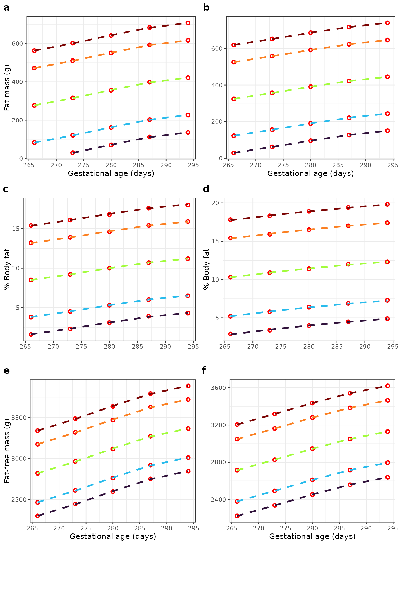
Observed and estimated normative centiles for body composition measures according to gestational age and sex. Centiles (3rd, 10th, 50th, 90th, and 97th) for fat mass (a males; b females); body fat percentage (c males; d females); and fat-free mass (e males; f females) according to gestational age. Red circles show the observed value for that centile and gestational age; dashed lines show estimates from linear equations fitted to these observed values.

Bland-Altman plots

Reference vs. predicted values

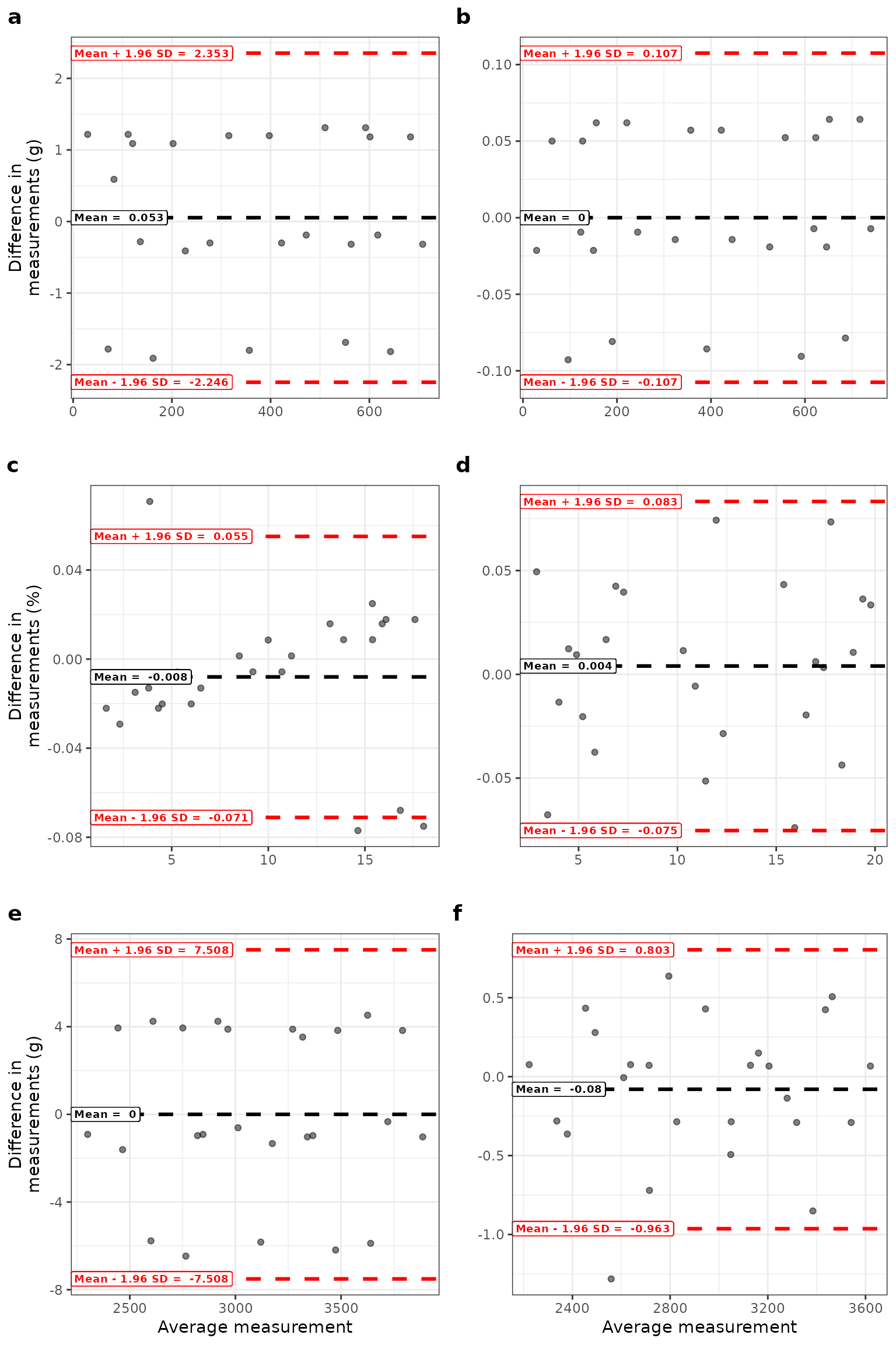
Bland-Altman plots for observed and estimated centile values for body composition measures according to gestational age and sex. Circles show differences between observed and estimated values for fat mass (a males; b females); body fat percentage (c males; d females); and fat-free mass (e males; f females) according to the average of the two measurements.

References

Villar J, Puglia FA, Fenton TR, Ismal LC, Staines-Urias E, Giuliani F, et al. Body composition at birth and its relationship with neonatal anthropometric ratios: the newborn body composition study of the INTERGROWTH-21st project Pediatric Research 2017, 82:305-316. doi: 10.1038/pr.2017.52