Blue Mountain Lake Polygon (Example Lake)

The OpenStreetMap boundary polygon for Blue Mountain Lake in Hamilton County, New York. Bundled with the package so that fetch examples can run offline (no internet or Overpass API call required) and pkgdown pages can render plot output. The coordinates match the sites in system.file("extdata", "sample_sites.csv", package = "lakefetch"), so the two datasets can be used together end-to-end.

Usage

example_lake

Format

An sf object with 1 row and 3 fields plus geometry:

osm_id

OSM relation identifier

name

Lake name ("Blue Mountain Lake")

area_km2

Surface area in square kilometers

geometry

MULTIPOLYGON geometry in UTM Zone 18N (EPSG:32618)

Source

Downloaded from OpenStreetMap https://www.openstreetmap.org/. See data-raw/create_example_data.R for the exact query.

Examples

data(example_lake)
print(example_lake)
#> Simple feature collection with 1 feature and 3 fields
#> Geometry type: POLYGON
#> Dimension:     XY
#> Bounding box:  xmin: 541565.8 ymin: 4855616 xmax: 545660 ymax: 4857845
#> Projected CRS: WGS 84 / UTM zone 18N
#>    osm_id               name area_km2                       geometry
#> 1 2202972 Blue Mountain Lake 5.055174 POLYGON ((543523.8 4857818,...

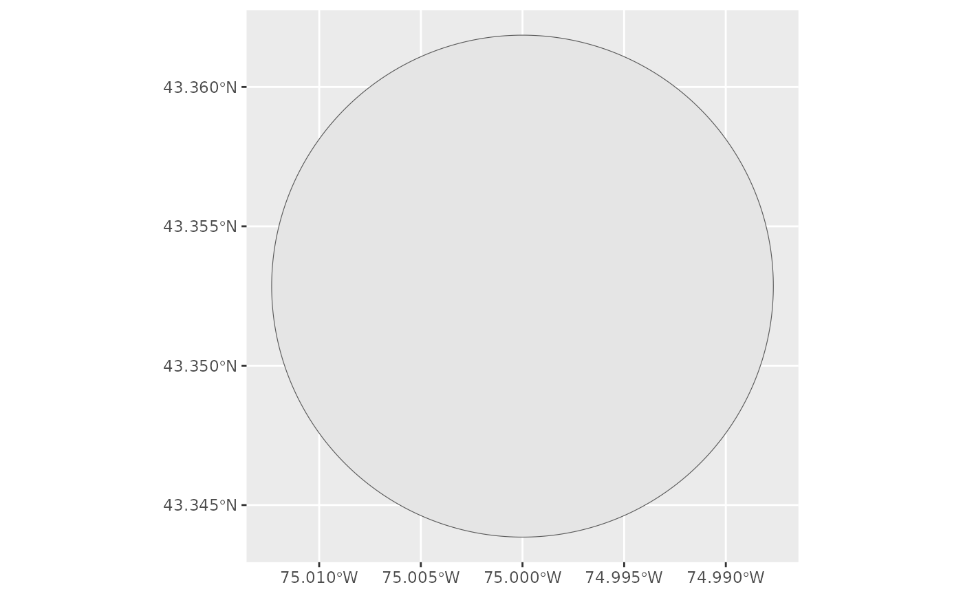
# Plot the lake
library(ggplot2)
ggplot(example_lake) + geom_sf()


# Load matching sample sites (they lie inside this polygon) and
# compute fetch end-to-end without touching OSM. First convert
# example_lake into the multi-lake list format that fetch_calculate()
# expects:
sites <- load_sites(system.file("extdata", "sample_sites.csv",
                                 package = "lakefetch"))
#> Loading data from: /github/home/R/x86_64-pc-linux-gnu-library/4.6/lakefetch/extdata/sample_sites.csv
#>   Loaded 2 rows with columns: Site, latitude, longitude, lake.name
#>   Using columns: Latitude = latitude, Longitude = longitude
#>   Preserved lake name column: lake.name
#>   Final valid samples: 2
#>   Detected location from column 'lake.name': Blue Mountain Lake
sites_sf <- sf::st_transform(
  sf::st_as_sf(sites, coords = c("longitude", "latitude"), crs = 4326,
               remove = FALSE),
  sf::st_crs(example_lake)
)
lake_data <- list(all_lakes = example_lake,
                  sites = sites_sf,
                  utm_epsg = sf::st_crs(example_lake)$epsg)
results <- fetch_calculate(sites, lake_data, add_context = FALSE)
#> Effective fetch method: top3
#> Using default depth: 10 m
#> Assigning sites to lakes...
#>   Checking direct intersections...
#>     2 sites matched directly
#>   Site assignment summary:
#>     Matched: 2/2
#>   Sites per lake:
#>     Blue Mountain Lake: 2 sites
#> Calculating fetch for multiple lakes...
#>   Buffering sites 10m inward
#>   Angle resolution: 5 degrees
#> Processing 1 lake(s)...
#> Using sequential processing
#>   Processing 2 samples in lake: Blue Mountain Lake
#> Fetch calculation complete.
sf::st_drop_geometry(results$results)[, c("Site", "fetch_effective",
                                           "exposure_category")]
#>     Site fetch_effective exposure_category
#> 1 BML1_1        2461.439         Sheltered
#> 2 BML2_2        2216.682         Sheltered