Plot Fetch Map

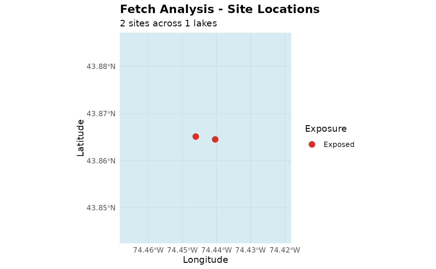
Create a map showing site locations colored by exposure category.

Usage

plot_fetch_map(fetch_data, title = "Fetch Analysis - Site Locations")

Arguments

fetch_data

Results from fetch_calculate

title

Optional plot title

Value

A ggplot2 object

Examples

# Use the bundled example lake (Blue Mountain Lake, NY) and the
# matching sample sites to compute and plot fetch offline.
data(example_lake)
sites_df <- load_sites(system.file("extdata", "sample_sites.csv",
                                    package = "lakefetch"))
#> Loading data from: /github/home/R/x86_64-pc-linux-gnu-library/4.6/lakefetch/extdata/sample_sites.csv
#>   Loaded 2 rows with columns: Site, latitude, longitude, lake.name
#>   Using columns: Latitude = latitude, Longitude = longitude
#>   Preserved lake name column: lake.name
#>   Final valid samples: 2
#>   Detected location from column 'lake.name': Blue Mountain Lake
sites_sf <- sf::st_transform(
  sf::st_as_sf(sites_df,
               coords = c("longitude", "latitude"), crs = 4326,
               remove = FALSE),
  sf::st_crs(example_lake)
)
lake_data <- list(all_lakes = example_lake,
                  sites = sites_sf,
                  utm_epsg = sf::st_crs(example_lake)$epsg)
results <- fetch_calculate(sites_df, lake_data, add_context = FALSE)
#> Effective fetch method: top3
#> Using default depth: 10 m
#> Assigning sites to lakes...
#>   Checking direct intersections...
#>     2 sites matched directly
#>   Site assignment summary:
#>     Matched: 2/2
#>   Sites per lake:
#>     Blue Mountain Lake: 2 sites
#> Calculating fetch for multiple lakes...
#>   Buffering sites 10m inward
#>   Angle resolution: 5 degrees
#> Processing 1 lake(s)...
#> Using sequential processing
#>   Processing 2 samples in lake: Blue Mountain Lake
#> Fetch calculation complete.
plot_fetch_map(results)