Advanced methods

Table of Contents

1. Working with non-animal/plant groups in phruta
2. Creating taxonomic constraints in phruta
3. Running PartitionFinder in phruta
4. Partitioned analyses in RAxML
5. Identifying rogue taxa

Working with non-animal nor plant groups in phruta

As explained in the brief intro to phruta, the sq.curate() function is primarily designed to curate taxonomic datasets using gbif. Alto gbif is extremely fast and efficient, it is largely designed to deal with animals and plants. If you’re interested in using the gbif backbone for curating sequence regardless of the kingdom use the following approach:

taxonomy.retrieve(species_names=c("Felis_catus", "PREDICTED:_Vulpes",
                  "Phoca_largha", "PREDICTED:_Phoca" ,
                  "PREDICTED:_Manis" , "Felis_silvestris" , "Felis_nigripes"),
                  database='gbif', kingdom=NULL)

Note that the kingdom argument is set to NULL. However, as indicated in the first vignette, gbif is efficient for retrieving accurate taxonomy when we provide details on the kingdom. Given that all the species we’re interested in are animals, we could just use:

taxonomy.retrieve(species_names=c("Felis_catus", "PREDICTED:_Vulpes",
                  "Phoca_largha", "PREDICTED:_Phoca" ,
                  "PREDICTED:_Manis" , "Felis_silvestris" , "Felis_nigripes"),
                  database='gbif', kingdom='animals')

We could also do the same for plants by using plants instead of animals in the kingdom argument. Now, what if we were interested in following other databases to retrieve taxonomic information for the species in our database? The latest version of phruta allow users to select the desired database. The databases follow the taxize::classification() function. Options are: ncbi, itis, eol, tropicos, nbn, worms, natserv, bold, wiki, and pow. Please select only one. Note that the gbif option in taxize::classification() is replaced by the internal gbif in phruta.

Now, let’s assume that we were interested in curating our database using itis:

taxonomy.retrieve(species_names=c("Felis_catus", "PREDICTED:_Vulpes",
                  "Phoca_largha", "PREDICTED:_Phoca" ,
                  "PREDICTED:_Manis" , "Felis_silvestris" , "Felis_nigripes"),
                  database='itis')

Using alternative databases is sometimes desirable. Please make sure you review which the best database is for your target group is before selecting one.

Creating taxonomic constraints in phruta

For different reasons, phylogenetic analyses sometimes require of tree constraints. phruta can automatically generate trees in accordance to taxonomy and a backbone topology. We divide constraint trees into two: (1) ingroup+outgroup and (2) particular clades.

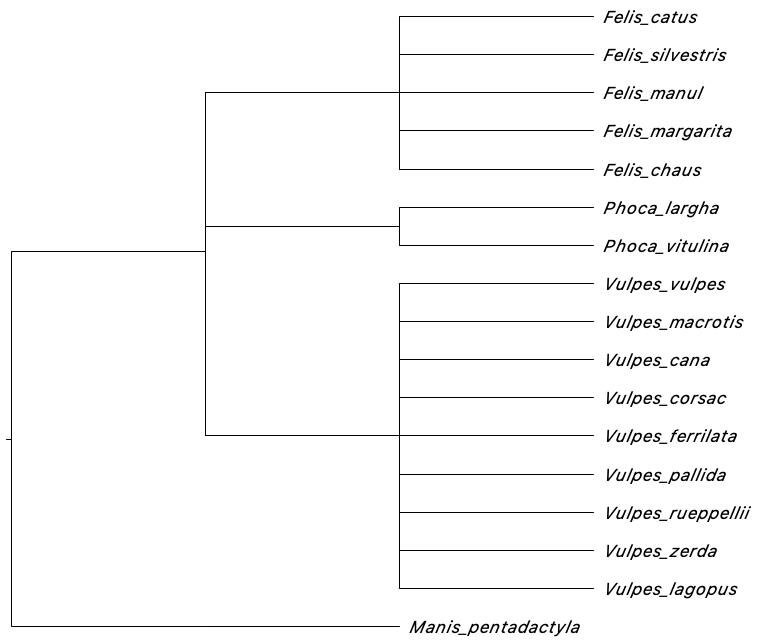
ingroup + outgroup

In this constraint type, phruta will create monophyletic groups for each of the taxonomic groups in the database (for selected target columns). Finally, it will generate tree with the same topology provided in the Topology argument. The user will provide the species names of the outgroup taxa as a vector of string that should fully match the names in the taxonomy file.

tree.constraint(
                taxonomy_folder = "1.CuratedSequences",
                targetColumns = c("kingdom", "phylum", "class", "order", 
                                  "family", "genus", "species_names"),
                Topology = "((ingroup), outgroup);",
                outgroup = "Manis_pentadactyla"
 )

Tree constraints ingroup+outgroup (example shown based on a much limited number of genes; see the examples in the package).

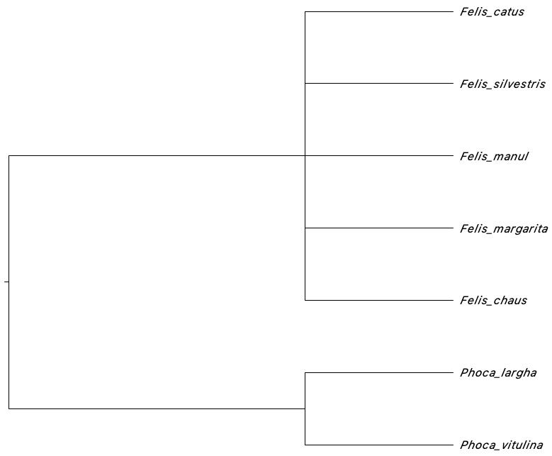
Particular clades

In this constraint type, phruta will create a constraint tree for particular clades. For instance, let’s assume that we only need to create a tree constraining the monophyly within two genera and their sister relationships:

tree.constraint( taxonomy_folder = "1.CuratedSequences",
                 targetColumns = c("kingdom", "phylum", "class", 
                                   "order", "family", "genus", "species_names"),
                 Topology = "((Felis), (Phoca));"
 )

Note that the key aspect in here is the Topology argument. It is a newick tree.

Tree constraints by clade (example shown based on a much limited number of genes; see the examples in the package).

Running PartitionFinder in phruta

With the current version of phruta, users are able to run PartitionFinder v1 within R. For this, users should provide the name of the folder where the alignments are stored, a particular pattern in the file names (masked in our case), and which models will be run in PartitionFinder. This function will download PartitionFinder, generate the input files, and run it all within R. The output files will be in a new folder within the working directory.

sq.partitionfinderv1(folderAlignments = "2.Alignments",
                    FilePatterns = "Masked",
                    models = "all"
 )

Unfortunately, the output files are not integrated with the current phruta pipeline. This will be part of a new release. However, users can still perform gene-based partitioned analyses within RAxML or can use PartitionFinder’s output files to inform their own analyses outside phruta.

Partitioned analyses in RAxML

Users can now run partitioned analyses in RAxML within phruta. This approach is implemented by setting the partitioned argument in tree.raxml to TRUE. For now, partitions are based on the genes are being analyzed. The same model is used to analyze each partition. More details on partitioned analyses can be customized by passing arguments in ips::raxml.

tree.raxml(folder = "2.Alignments", FilePatterns = "Masked",
           raxml_exec = "raxmlHPC", Bootstrap = 100,
           outgroup = "Manis_pentadactyla",
           partitioned=T
)

Identifying rogue taxa

phruta can help users run RogueNaRok implemented in the Rogue R package. Users can then examine whether rogue taxa should be excluded from the analyses. tree.roguetaxa() uses the bootstrap trees generated using the tree.raxml() function along with the associated best tree to identify rogue taxa.

tree.roguetaxa(folder = "3.Phylogeny")