Create a species-area relationship (SAR) plot

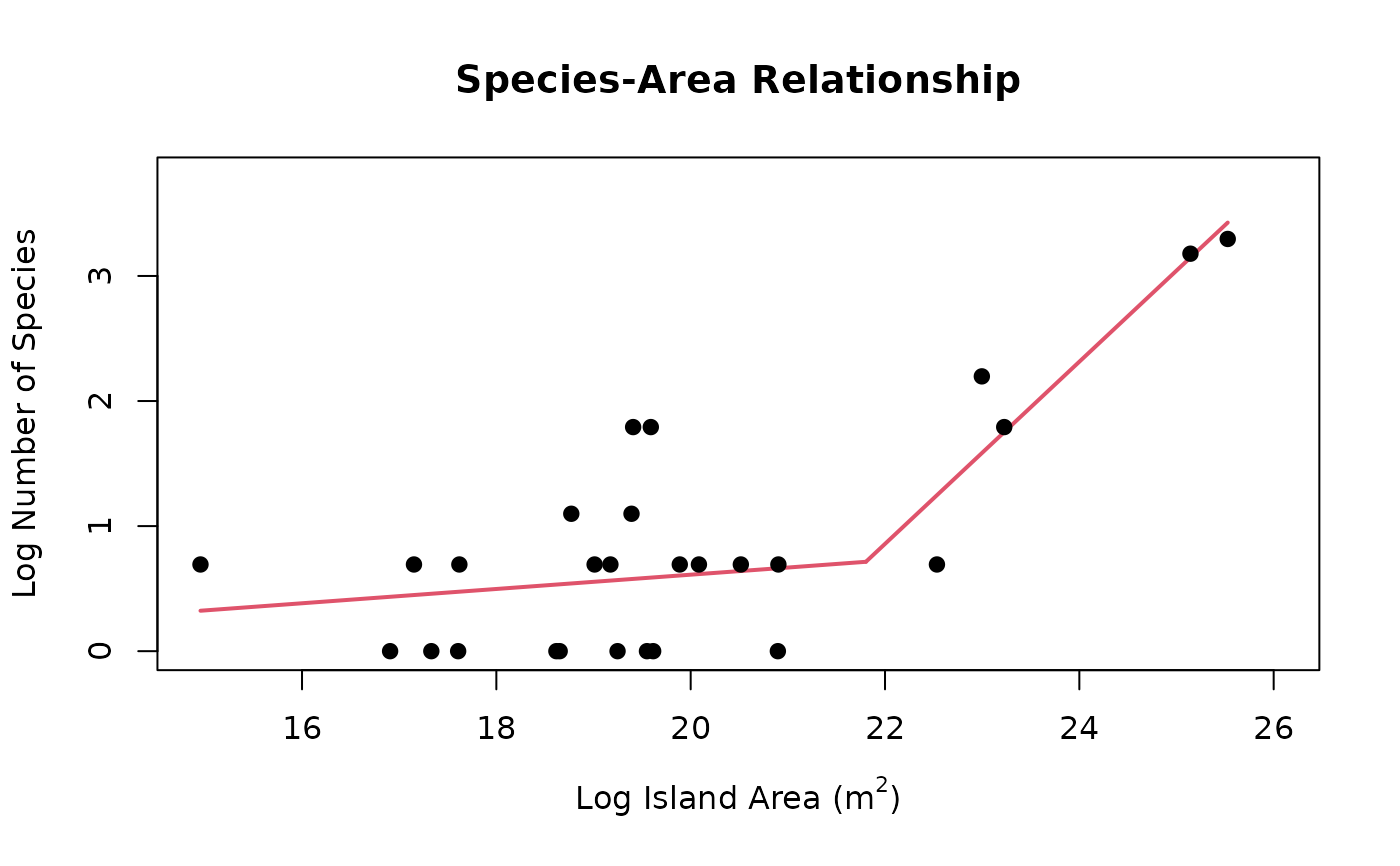
Use segmented regression to create a species-area relationship (SAR) plot. The X axis represents log(island area) and the Y axis represents log(number of species)

Usage

create_sar(occurrences, npsi = 1, visualize = FALSE)

create_SAR(occurrences, npsi = 1, visualize = FALSE)

Arguments

occurrences

The dataframe output by ssarp::find_areas() (or if using a custom dataframe, ensure that it has the following columns: specificEpithet, areas)

npsi

The maximum number of breakpoints to estimate for model selection. Default: 1

visualize

(boolean) Whether the plot should be displayed when the function is called. Default: FALSE

Value

A list of class SAR with 5 items including:

• summary: the summary output

• segObj or linObj: the regression object (segObj when segmented, linObj when linear)

• aggDF: the aggregated dataframe used to create the plot

• AICscores: the AIC scores generated during model selection

• AllModels: a list of models created in model selection, labeled by number of breakpoints

Details

If the user would prefer to create their own plot of the ssarp::create_sar() output, the aggDF element of the returned list includes the raw points from the plot created here. They can be accessed as demonstrated in the Examples section.

Examples

# The GBIF key for the Anolis genus is 8782549
# Read in example dataset filtered from:
#  dat <- rgbif::occ_search(taxonKey = 8782549,
#                           hasCoordinate = TRUE,
#                           limit = 10000)
dat <- read.csv(system.file("extdata",
                            "ssarp_Example_Dat.csv",
                            package = "ssarp"))
land <- find_land(occurrences = dat)
areas <- find_areas(occs = land)
#> ℹ Recording island names...
#> ℹ Assembling island dictionary...
#> ℹ Adding areas to final dataframe...

seg <- create_sar(occurrences = areas,
                  npsi = 1,
                  visualize = FALSE)
plot(seg)

summary <- seg$summary
model_object <- seg$segObj
points <- seg$aggDF