About rangr
This vignette shows an example of a basic use of the
rangr package. The main goal of this tool is to simulate
species range dynamics. The simulations can be performed in a spatially
explicit and dynamic environment, allowing for projections of how
populations will respond to e.g. climate or land use changes.
Additionally, by implementing various sampling methods and observational
error distributions, it can accurately reflect the structure of original
survey data or simulate random sampling.
Here, we showcase the full capabilities of our package, from creating a virtual species to performing simulation and visualization of results.
Basic workflow
In this chapter we will show you how to perform basic simulation using maps provided with the package.
Installing the package
First we need to install and load the rangr package.
install.packages("rangr")
library(rangr)
Since the maps in which the simulation takes place have to be in the
SpatRaster format, we will also install and load the
terra package to facilitate their manipulation and
visualisation.
install.packages("terra")
library(terra)
Input maps
One of the most important input parameters for simulation are maps specifying the abundance of the virtual species at the starting point of the simulation and carrying capacity of environment in which simulation takes place. In this section, we will not generate them from scratch. Instead, we will use maps provided with the package.
Example maps available in rangr in the Cartesian coordinate system:
n1_small.tifn1_big.tifK_small.tifK_small_changing.tifK_big.tif
Example maps available in rangr in the longitude/latitude coordinate system:
n1_small_lon_lat.tifn1_big_lon_lat.tifK_small_lon_lat.tifK_small_changing_lon_lat.tifK_big_lon_lat.tif
You can find additional information about these data sets in help files:
?n1_small.tif
?K_small.tif
We will use these two datasets right now:
n1_small.tif- as abundance at the starting point,K_small.tif- as carrying capacity.
To read the data we can use rast function from the
terra package:
n1_small <- rast(system.file("input_maps/n1_small.tif", package = "rangr"))
K_small <-  rast(system.file("input_maps/K_small.tif", package = "rangr"))
Since both of these maps refer to the same virtual or in this case real environment (a small region located in northwestern Poland), they must have the same dimensions, resolution, geographical projection etc. The only differences between them may be the values they contain and the number of layers. You can use multiple layers in the carrying capacity map to create a dynamic environment during the simulation, but in this example, we will demonstrate a static environment.
Let’s take a closer look at them:
n1_small
#> class       : SpatRaster
#> size        : 15, 10, 1  (nrow, ncol, nlyr)
#> resolution  : 1000, 1000  (x, y)
#> extent      : 270000, 280000, 610000, 625000  (xmin, xmax, ymin, ymax)
#> coord. ref. : ETRS89 / Poland CS92
#> source      : n1_small.tif
#> name        : layer
#> min value   :     0
#> max value   :    10
K_small
#> class       : SpatRaster
#> size        : 15, 10, 1  (nrow, ncol, nlyr)
#> resolution  : 1000, 1000  (x, y)
#> extent      : 270000, 280000, 610000, 625000  (xmin, xmax, ymin, ymax)
#> coord. ref. : ETRS89 / Poland CS92
#> source      : K_small.tif
#> name        : layer
#> min value   :     0
#> max value   :   100
Above, you can see the dimensions and other basic characteristics of the sample maps. The only field that differs between these maps is the value field.
Now we will use the plot function to visualise input
maps to get an even better idea of what we’re working with.
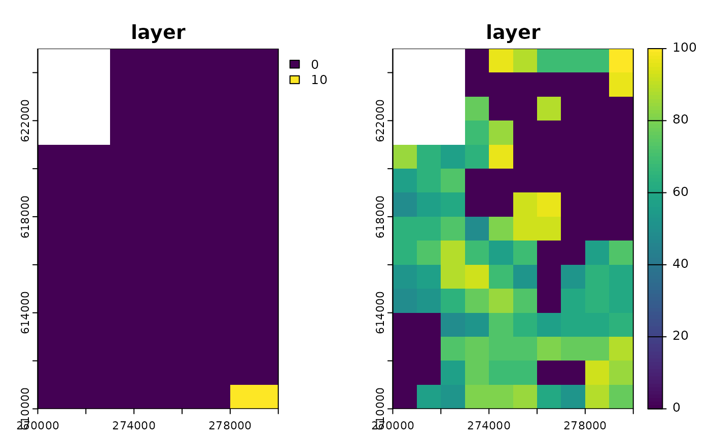
Input maps
Several things are noticeable here:
The shape is the same for both maps, and in both cases, the upper left corner of the map is excluded from the simulation area and is treated as if it were outside the map’s extent. To create such an irregular shape,
NAmust be assigned to a particular cell or group of cells.The initial population is only located in the lower right corner of the simulation area and occupies two cells. Each of them contains 10 individuals (you can use the
values()function to check).The carrying capacity map has areas that are unsuitable for the presented virtual species, as well as areas where it can have a positive population growth rate.
Initialise
Now that we have input maps, we will use the
initialise() function to set other input parameters and
generate a sim_data object that will contain all the
necessary information to perform a simulation.
The most basic initialise() call will look as
follows:
sim_data_01 <- initialise(
  n1_map = n1_small,
  K_map = K_small,
  r = log(2),
  rate = 1 / 1e3
)
Let’s break down this command:
n1_mapandK_maprefer to the input maps described earlier.The
rparameter is used to set the intrinsic population growth rate. The default population growth function is the Gompetz function.The
rateparameter is related to thekernel_funparameter, which by default is set to an exponential function (rexp). Therefore,ratedetermines the shape of the dispersal kernel (the mean dispersal distance is 1/rate).
We have now set up the simulation environment along with the demographic and dispersal processes. This is the most basic setup needed to run your first simulation, and that’s what we’ll do in the next step.
But first, let’s see what other information sim_data
contains and what happened behind the scenes during initialisation.
First, let’s check the class of sim_data object:
class(sim_data_01)
#> [1] "sim_data" "list"
As you can see sim_data is a sim_data
object that inherits from list objects so it is possible to
change values of this object by hand. However, we strongly encourage you
to use update() function instead to avoid errors and
problems with data integration.
To take a closer look at sim_data you can also use
print() or summary() function:
summary(sim_data_01)
#> Summary of sim_data object
#>
#> n1 map summary:
#>    Min. 1st Qu.  Median    Mean 3rd Qu.    Max.     NAs
#>  0.0000  0.0000  0.0000  0.1449  0.0000 10.0000      12
#>
#> Carrying capacity map summary:
#>    Min. 1st Qu.  Median    Mean 3rd Qu.    Max.     NAs
#>    0.00    0.00   56.00   44.84   72.00  100.00      12
#>
#> growth        gompertz
#> r               0.6931
#> A                    -
#> kernel_fun        rexp
#> dens_dep           K2N
#> border       absorbing
#> max_dist          2000
#> changing_env     FALSE
#> dlist             TRUE
It will show the summary of both input maps, as well as list of other
most important parameters such as r that we set up
earlier.
Simulation
All you need to run a simulation is a sim_data object
and a specified number of time steps to simulate. In addition, you can
use the burn parameter to discard a selected number of
initial time steps if this makes sense for your research or
experiment.
In this first example, we will only set the time
parameter as we want to observe how our virtual species disperses and
reproduces.
sim_result_01 <- sim(obj = sim_data_01, time = 100)Again we will check the class of returned object:
class(sim_result_01)
#> [1] "sim_results" "list"
Similar to initialise, sim also returns an
object that inherits from list, but in this case it is
called sim_results. This list has 3 elements such as:
extinction-TRUEif the population is extinct orFALSEotherwisesimulated_time- number of simulated time steps without the burn-inN_map- 3-dimensional array representing the spatiotemporal variability of population numbers. The first two dimensions correspond to the spatial aspect of the output and the third dimension represents time.
The best way to take a closer look at the results is to call a summary function.
summary(sim_result_01)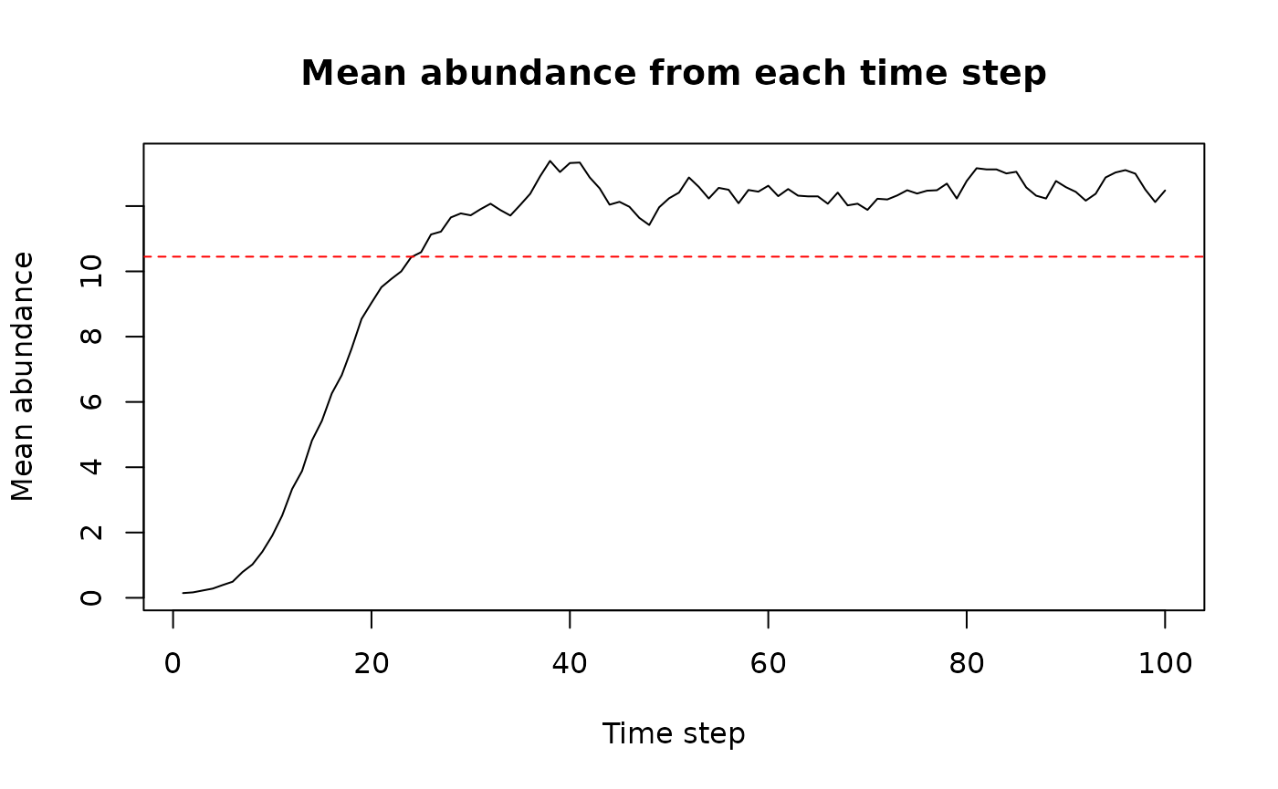
#> Summary of sim_results object
#>
#> Simulation summary:
#>
#> simulated time   100
#> extinction     FALSE
#>
#> Abundances summary:
#>    Min. 1st Qu.  Median    Mean 3rd Qu.    Max.     NAs
#>    0.00    0.00   12.00   10.45   19.00   54.00    1200
It gives you a quick and easy overview of the simulation results by
providing simulation time, extinction status and a summary of all maps
with abundances. It also produces a plot which can be useful for
determining the value of the burn parameter.
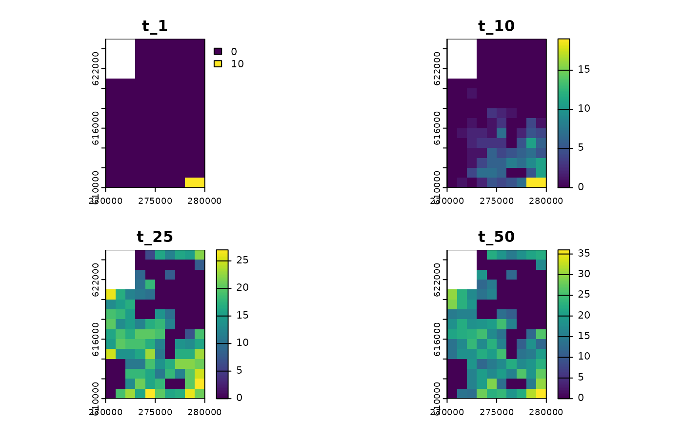
Visualisation
With rangr we have provided an easy way to visualise
selected time steps from the simulation. This can be done using the
generic plot function:
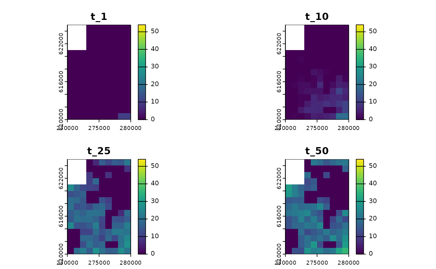
Abundances
#> class       : SpatRaster
#> size        : 15, 10, 4  (nrow, ncol, nlyr)
#> resolution  : 1000, 1000  (x, y)
#> extent      : 270000, 280000, 610000, 625000  (xmin, xmax, ymin, ymax)
#> coord. ref. : ETRS89 / Poland CS92
#> source(s)   : memory
#> names       : t_1, t_10, t_25, t_50
#> min values  :   0,    0,    0,    0
#> max values  :  10,   19,   27,   36
You can also adjust its parameters to get more breaks on the color scale:
plot(sim_result_01,
  time_points = c(1, 10, 25, 50),
  breaks = seq(0, max(sim_result_01$N_map + 5, na.rm = TRUE), by = 5),
  template = sim_data_01$K_map
)
Abundances
#> class       : SpatRaster
#> size        : 15, 10, 4  (nrow, ncol, nlyr)
#> resolution  : 1000, 1000  (x, y)
#> extent      : 270000, 280000, 610000, 625000  (xmin, xmax, ymin, ymax)
#> coord. ref. : ETRS89 / Poland CS92
#> source(s)   : memory
#> names       : t_1, t_10, t_25, t_50
#> min values  :   0,    0,    0,    0
#> max values  :  10,   19,   27,   36
If you prefer to work with rasters, you can also convert any
sim_result object into SpatRaster using the
to_rast() function:
# raster construction
my_rast <- to_rast(
  sim_result_01,
  time_points = 1:sim_result_01$simulated_time,
  template = sim_data_01$K_map
)

# print raster
my_rast
#> class       : SpatRaster
#> size        : 15, 10, 100  (nrow, ncol, nlyr)
#> resolution  : 1000, 1000  (x, y)
#> extent      : 270000, 280000, 610000, 625000  (xmin, xmax, ymin, ymax)
#> coord. ref. : ETRS89 / Poland CS92
#> source(s)   : memory
#> names       : t_1, t_2, t_3, t_4, t_5, t_6, ...
#> min values  :   0,   0,   0,   0,   0,   0, ...
#> max values  :  10,  11,  14,  16,  20,  13, ...
And then visualise it using the plot() function:
Abundances
Virtual Ecologist
If you want to sample the abundance of your virtual species
population and mimic the observation process, you can use the
get_observations() function. Depending on the
type argument, observation sites can be selected randomly
or their coordinates can be provided as a data.frame.
Here we will demonstrate the most basic variant of the
get_observations() function. To do this we will need both
the sim_results object and the sim_data object
used to generate the simulated data. We will randomly select observation
sites, and in this variant we need to specify what proportion of all
sites we want to make observations on. Here we will select 10% of the
sites, so the prop argument is set to 0.1. There are two
random observation processes available: one where the observation sites
are the same at all time steps, and the other where the observation
sites are different at each time step. To see how the first version
works, we set the type argument to
"random_one_layer".
set.seed(123)
sample_01 <- get_observations(
   sim_data_01,
   sim_result_01,
   type = "random_one_layer",
   prop = 0.1
)
str(sample_01)
#> 'data.frame':    1500 obs. of  4 variables:
#>  $ x        : num  279500 271500 279500 274500 279500 ...
#>  $ y        : num  623500 618500 612500 619500 610500 ...
#>  $ time_step: int  1 1 1 1 1 1 1 1 1 1 ...
#>  $ n        : num  0 0 0 0 10 0 0 0 0 0 ...
The returned data.frame contains the geodetic
coordinates of the survey sites, the population abundances, and the time
steps from which the abundances were observed. To confirm that the
survey sites remain the same in each time step, and to obtain the
coordinates of these sites, we can use the following code:
unique(sample_01[c("x", "y")])
#>         x      y
#> 1  279500 623500
#> 2  271500 618500
#> 3  279500 612500
#> 4  274500 619500
#> 5  279500 610500
#> 6  277500 610500
#> 7  271500 614500
#> 8  272500 614500
#> 9  272500 610500
#> 10 273500 614500
#> 11 272500 611500
#> 12 274500 623500
#> 13 274500 614500
#> 14 270500 613500
#> 15 273500 616500
Here we sampled 15 sites.
The observation process is not perfect due to, among other things,
the detectability of the species or the skill of the observer. To mimic
this, we need to set obs_error and
obs_error_param arguments, which set the level of random
noise in the observation process generated from the log-normal
distribution or the binomial distribution. Here we will use the first
one.
sample_01 <- get_observations(
   sim_data_01,
   sim_result_01,
   type = "random_one_layer",
   prop = 0.1,
   obs_error = "rlnorm",
   obs_error_param = log(1.2)
)
Now let’s demonstrate the second random observation process. We will
set the type argument to "random_all_layers".
This version ensures that the study sites are re-sampled at each time
step.
set.seed(123)
sample_02 <- get_observations(
   sim_data_01,
   sim_result_01,
   type = "random_all_layer",
   prop = 0.1,
   obs_error = "rlnorm",
   obs_error_param = log(1.2)
)
Let’s have a look which observation sites were sampled this time.
Here we looked at 138 observed sites (all available), each of which was “visited” at least once.
More advanced workflow
The previous workflow was quite basic. Now we will present a more advanced one and use it to show some of the other parameter options.
Input maps
Abundances at the first time step
As mentioned earlier, rangr has the ability to simulate
virtual species in a changing environment, and in this example we will
show you how to do this. For a better illustration we should start with
a more populated map than the n1_small used before. The
easiest way to do this is to use the abundances from the last time step
of the previous simulation as input for the current one. This can be
done as follows:
n1_small_02 <- n1_small
values(n1_small_02) <- (sim_result_01$N_map[, , 100])
Carrying capacity
To simulate a changing environment, we need to specify the changes we
want. Essentially you need a carrying capacity map for each time step of
the simulation. You can generate these yourself, or you can generate
maps only for a few key time steps (at least the first and last) and
then use K_get_interpolation() to generate the missing
ones. Here we will choose the second option and use the
K_small_changing object that comes with rangr.
Below you can see its summary:
K_small_changing <- rast(system.file("input_maps/K_small_changing.tif",
                                     package = "rangr"))
K_small_changing
#> class       : SpatRaster
#> size        : 15, 10, 3  (nrow, ncol, nlyr)
#> resolution  : 1000, 1000  (x, y)
#> extent      : 270000, 280000, 610000, 625000  (xmin, xmax, ymin, ymax)
#> coord. ref. : ETRS89 / Poland CS92
#> source      : K_small_changing.tif
#> names       : layer.1, layer.2, layer.3
#> min values  :       0,       0,       0
#> max values  :     100,     130,     170
As you can see, the carrying capacity increases in each map, meaning
that our environment is becoming more and more suitable for the virtual
species. It is also worth noting that the first layer of
K_small_changing is the same as K_small.
Again, we can visualise all the input maps using the plot function:
plot(c(n1_small_02, K_small_changing),
     range = range(values(c(n1_small_02, K_small_changing)), na.rm = TRUE),
     main = c("n1", paste0("K", 1:nlyr(K_small_changing))))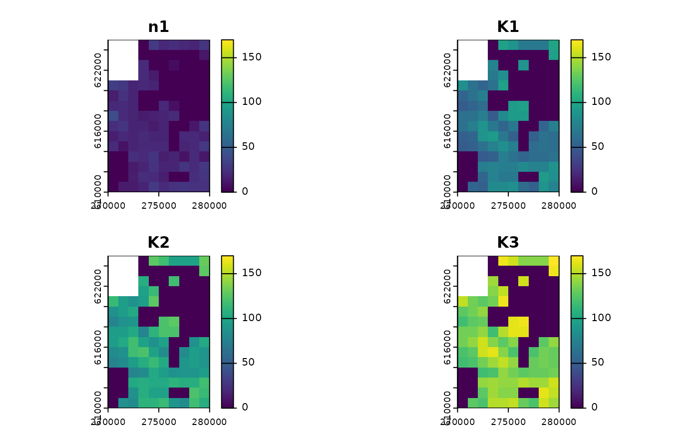
Input maps
This raster has 3 layers so we can either run a simulation with only
3 time steps (which seems rather pointless) or, as mentioned, use the
K_get_interpolation() function to generate maps for each
time step. In this example, we will do 200 time steps so we will need
200 maps.
The first and last layers from K_small_changing
correspond to the first and last time steps and the middle layer can be
assigned to any time step in between. In addition, to give our virtual
species some time to adapt to the new parameters, the first few carrying
capacity maps will be the same. This is done by duplicating the first
layer of K_small_changing. Therefore, the layers and
corresponding time points will be as follows:
1st layer of
K_small_changing- 1st time step,duplicated 1st layer of
K_small_changing- 20th time step,2nd layer of
K_small_changing- 80th time step,3rd layer of
K_small_changing- 200th time step.
This translates into a stable environment during 1-20 time steps, a rapidly increasing carrying capacity during 20-80 time steps and slowly rising carrying capacity during 80-200 time steps.
# duplicate 1st layer of K_small_changing
K_small_changing_altered <- c(K_small, K_small_changing)

# interpolate to generate maps for each time step
K_small_changing_interpolated <- K_get_interpolation(
  K_small_changing_altered,
  K_time_points = c(1, 20, 80, 200))
#> Warning in K_check(K_map, K_time_points, time): Argument "time" is no specified
#> - maximum from "K_time_points" is used as "time"
K_small_changing_interpolated
#> class       : SpatRaster
#> size        : 15, 10, 200  (nrow, ncol, nlyr)
#> resolution  : 1000, 1000  (x, y)
#> extent      : 270000, 280000, 610000, 625000  (xmin, xmax, ymin, ymax)
#> coord. ref. : ETRS89 / Poland CS92
#> source(s)   : memory
#> names       : lyr.1, lyr.2, lyr.3, lyr.4, lyr.5, lyr.6, ...
#> min values  :     0,     0,     0,     0,     0,     0, ...
#> max values  :   100,   100,   100,   100,   100,   100, ...
# visualise results
vis_layers <- c(1, 20, 30, seq(50, 200, by = 20), 200)
plot(subset(K_small_changing_interpolated, subset = vis_layers),
     range = range(values(K_small_changing_interpolated), na.rm = TRUE),
     main = paste0("K", vis_layers),
)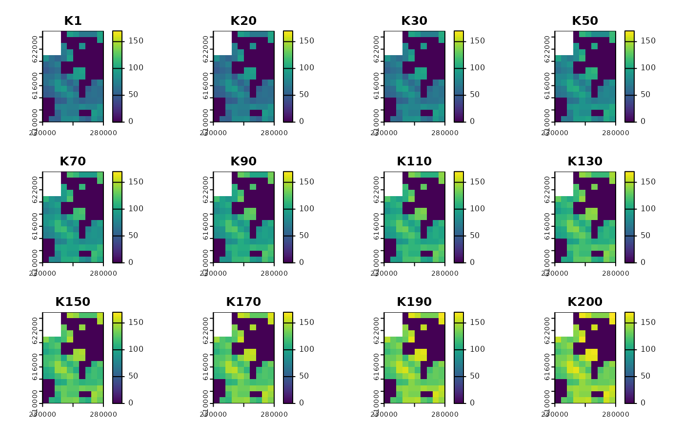
Interpolation results
This completes the preparation of the input maps required for this example. We will now select values for other parameters.
Initialise (using update function)
First, let’s take a look at the sim_data object from the
previous chapter:
sim_data_01
#> Class: sim_data
#>
#> n1_map:
#>    Min. 1st Qu.  Median    Mean 3rd Qu.    Max.     NAs
#>  0.0000  0.0000  0.0000  0.1449  0.0000 10.0000      12
#>
#> K_map:
#> class       : SpatRaster
#> size        : 15, 10, 1  (nrow, ncol, nlyr)
#> resolution  : 1000, 1000  (x, y)
#> extent      : 270000, 280000, 610000, 625000  (xmin, xmax, ymin, ymax)
#> coord. ref. : ETRS89 / Poland CS92
#> source(s)   : memory
#> name        : layer
#> min value   :     0
#> max value   :   100
#>
#> resolution              1000
#> r          0.693147180559945
#> r_sd                       0
#> K_sd                       0
#> growth              gompertz
#> A                          -
#> dens_dep                 K2N
#> border             absorbing
#> max_dist                2000
#> kernel_fun              rexp
#> dlist                   TRUE
After the information about the input maps, we can see a list of parameters that can be modified. We will change the following:
r- intrinsic growth rate,r_sd- intrinsic growth rate stochasticity,K_sd- environmental stochasticity,growth- growth function of virtual species,A- strength of the Allee effect,dens_dep- what determines the possibility of settling in particular cell,border- how borders are treated.
To change these parameters (along with the carrying capacity map
prepared in the previous section), we could simply initialise a new
sim_data object from scratch. Here we will use
update() on sim_data from the previous example
to demonstrate its use.
sim_data_02 <- update(sim_data_01,
  n1_map = K_small,
  K_map = K_small_changing_interpolated,
  K_sd = 0.1,
  r = log(5),
  r_sd = 0.05,
  growth = "ricker",
  A = 0.2,
  dens_dep = "K",
  border = "reprising",
  rate = 1 / 500
)
The growth of virtual species is now defined using the Ricker
function (growth = "ricker") with increased intrinsic
growth rate (r = log(5)) combined
with weak Allee effect (A = 0.2) and added demographic
stochasticity (r_sd = 0.05). The probability of settlement
in a target cell is determined solely by its carrying capacity value
(dens_dep = "K"). We also changed the parameter of a
dispersal kernel (rate = 1/500) and the behaviour of the
species near the borders - now specimens cannot leave the specified
study area (border = "reprising").
sim_data_02
#> Class: sim_data
#>
#> n1_map:
#>    Min. 1st Qu.  Median    Mean 3rd Qu.    Max.     NAs
#>    0.00    0.00   56.00   44.84   72.00  100.00      12
#>
#> K_map:
#> class       : SpatRaster
#> size        : 15, 10, 200  (nrow, ncol, nlyr)
#> resolution  : 1000, 1000  (x, y)
#> extent      : 270000, 280000, 610000, 625000  (xmin, xmax, ymin, ymax)
#> coord. ref. : ETRS89 / Poland CS92
#> source(s)   : memory
#> names       :     lyr.1,    lyr.2,      lyr.3,      lyr.4,      lyr.5,      lyr.6, ...
#> min values  :         0,        0,          0,          0,          0,          0, ...
#> max values  : 98.978292, 104.7768, 124.106876, 110.654446, 138.736246, 113.891581, ...
#>
#> resolution            1000
#> r          1.6094379124341
#> r_sd                  0.05
#> K_sd                   1.1
#> growth              ricker
#> A                      0.2
#> dens_dep                 K
#> border           reprising
#> max_dist              1000
#> kernel_fun            rexp
#> dlist                 TRUE
Simulation
The simulation setup will be very similar to the previous one. We have designed it this way to simplify the process of simulation replication. We will also now demonstrate how parallel computing can be used when running simulations:
library(parallel)
cl <- makeCluster(detectCores() - 2)

sim_result_02 <-
  sim(obj = sim_data_02, time = 200, cl = cl)

stopCluster(cl)
summary(sim_result_02)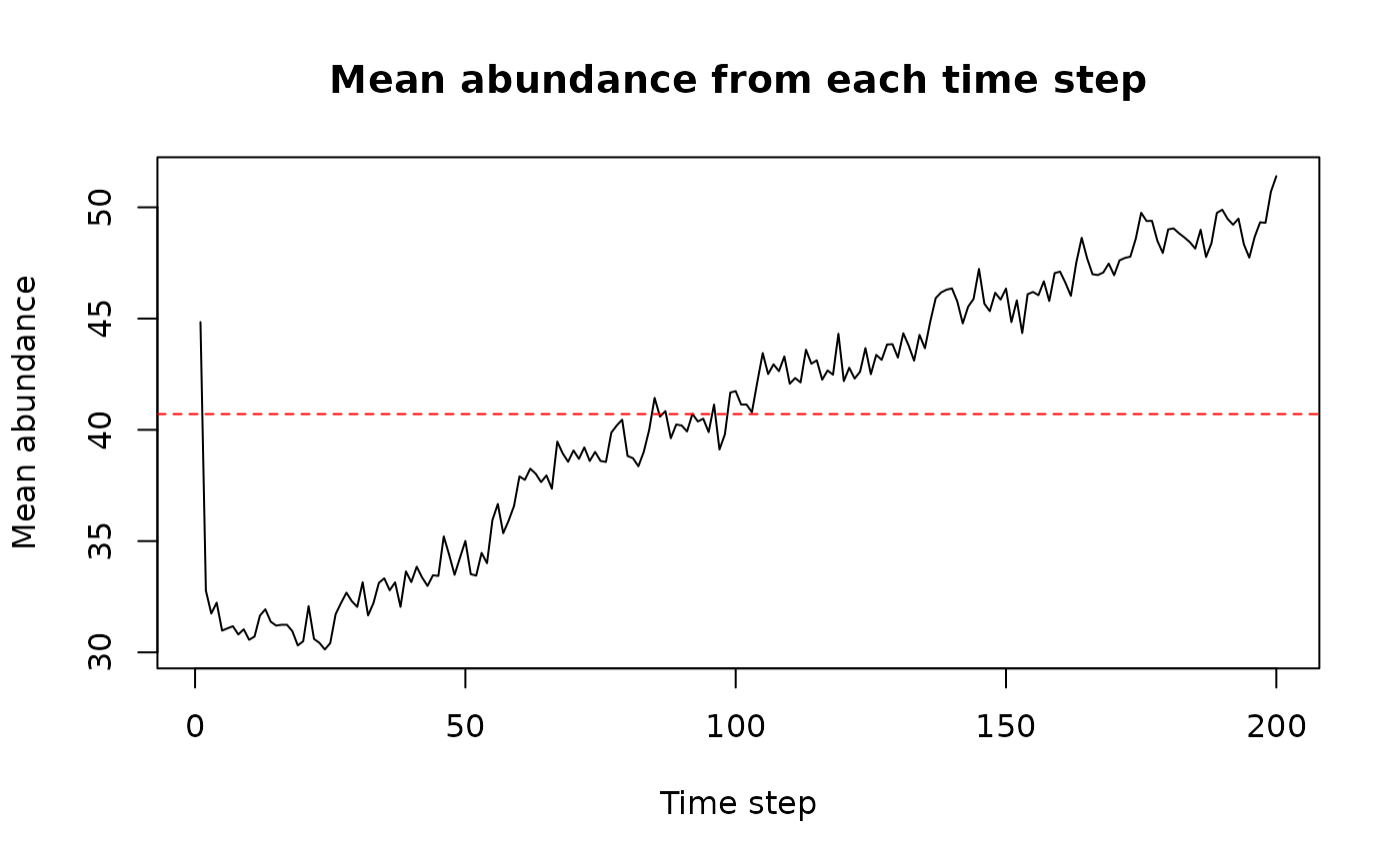
#> Summary of sim_results object
#>
#> Simulation summary:
#>
#> simulated time   200
#> extinction     FALSE
#>
#> Abundances summary:
#>    Min. 1st Qu.  Median    Mean 3rd Qu.    Max.     NAs
#>    0.00    0.00   47.00   40.71   72.00  148.00    2400
The behaviour of the virtual species created and the world in which it lives is now much more complex than before. As a result, it can better mimic real ecological scenarios that users may wish to explore. In this case, we observe a decrease in mean abundance in the first few time steps of the simulation due to a change in parameters from the previous simulation. Then we see a rapidly increasing trend to catch up with the increasing carrying capacity, which slows down slightly later.
Visualisation
Let’s visualise the result of this simulation.
plot(sim_result_02,
  time_points = c(1, 10, seq(20, 200, by = 20)),
  breaks = seq(0, max(sim_result_02$N_map + 5, na.rm = TRUE), by = 20),
  template = sim_data_02$K_map
)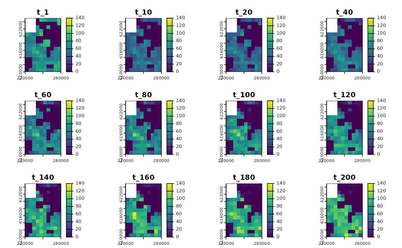
Abundances
#> class       : SpatRaster
#> size        : 15, 10, 12  (nrow, ncol, nlyr)
#> resolution  : 1000, 1000  (x, y)
#> extent      : 270000, 280000, 610000, 625000  (xmin, xmax, ymin, ymax)
#> coord. ref. : ETRS89 / Poland CS92
#> source(s)   : memory
#> names       : t_1, t_10, t_20, t_40, t_60, t_80, ...
#> min values  :   0,    0,    0,    0,    0,    0, ...
#> max values  : 100,   72,   75,   78,  107,  114, ...
Virtual Ecologist
Here we present two other ways to simulate the observation process
using simulated abundances and the get_observations()
function.
The first way is to provide the coordinates of the sample sites and
the time steps in which the observation is to take place. This should be
provided in the form of a data.frame with three columns:
“x”, “y” and “time_step”. We have provided an example of such a data
frame with rangr - it is used in code examples by the package, but here
we will create one from scratch, as the one provided only considers 100
time steps (not 200, which we need now). We will use the same
observation sites for each time step.
set.seed(123)
str(observations_points) # required structure
#> 'data.frame':    1500 obs. of  3 variables:
#>  $ x        : int  277500 276500 274500 274500 279500 278500 272500 273500 272500 278500 ...
#>  $ y        : int  622500 614500 610500 614500 613500 619500 618500 613500 616500 623500 ...
#>  $ time_step: int  1 1 1 1 1 1 1 1 1 1 ...

all_coords <- crds(sim_data_02$K_map)
observations_coords <-
  all_coords[sample(1:nrow(all_coords), 0.1 * nrow(all_coords)),]
time_steps <- sim_result_02$simulated_time
ncells <- nrow(observations_coords)

points <- data.frame(
    x = rep(observations_coords[, "x"], times = time_steps),
    y = rep(observations_coords[, "y"], times = time_steps),
    time_step = rep(1:time_steps, each = ncells)
  )
str(points)
#> 'data.frame':    2600 obs. of  3 variables:
#>  $ x        : num  279500 271500 279500 274500 279500 ...
#>  $ y        : num  623500 618500 612500 619500 610500 ...
#>  $ time_step: int  1 1 1 1 1 1 1 1 1 1 ...
We can see that for each data (study site and time step) an observation has been made and is now stored in the “n” column.
Now that we have selected study sites along with time steps, we can
pass this data to the get_observations() function.
set.seed(123)

sample_03 <- get_observations(
  sim_data_02,
  sim_result_02,
  type = "from_data",
  points = points,
  obs_error = "rlnorm",
  obs_error_param = log(1.2)
)
str(sample_03)
#> 'data.frame':    2600 obs. of  4 variables:
#>  $ x        : num  279500 271500 279500 274500 279500 ...
#>  $ y        : num  623500 618500 612500 619500 610500 ...
#>  $ time_step: int  1 1 1 1 1 1 1 1 1 1 ...
#>  $ n        : num  86.7 53.7 116.9 0 77 ...
We will now demonstrate the latest (for now) version of the
get_observations() function. It is designed to simulate
real monitoring surveys by mimicking the observation process based on
its statistical properties. Whether a survey is made by the same
observer for several years or not is defined by a geometric distribution
(rgeom). The study sites available to virtual observers are
passed using the cells_coords argument. We will use the
sites sampled in the previous example, stored in the
observations_coords variable, as they are already in the
required format (data.frame with ‘x’ and ‘y’ columns).
set.seed(123)

sample_04 <- get_observations(
  sim_data_02,
  sim_result_02,
  type = "monitoring_based",
  cells_coords = observations_coords,
  obs_error = "rlnorm",
  obs_error_param = log(1.2)
)
str(sample_04)
#> 'data.frame':    2251 obs. of  5 variables:
#>  $ x        : num  279500 279500 279500 279500 279500 ...
#>  $ y        : num  623500 623500 623500 623500 623500 ...
#>  $ time_step: int  1 2 3 4 5 6 7 8 11 12 ...
#>  $ obs_id   : chr  "obs1" "obs1" "obs1" "obs2" ...
#>  $ n        : num  109.1 79.6 58.5 34.3 48.8 ...
length(unique(sample_04$obs_id))
#> [1] 62
Here we can see that 62 unique observers made ‘observations’. For
each study site, the first observer identifier is set to “obs1”, the
second to “obs2” and so on. The time that an observer would survey the
same site, as well as the probability of making any observations at all,
is defined by a geometric distribution. We can change the shape of this
distribution using the prob argument. It is set to 0.3 by
default, and we will now set it to 0.2 to see how this affects the
number of unique observers.
set.seed(123)

sample_04 <- get_observations(
  sim_data_02,
  sim_result_02,
  type = "monitoring_based",
  cells_coords = observations_coords,
  obs_error = "rlnorm",
  obs_error_param = log(1.2),
  prob = 0.2
)
str(sample_04)
#> 'data.frame':    2454 obs. of  5 variables:
#>  $ x        : num  279500 279500 279500 279500 279500 ...
#>  $ y        : num  623500 623500 623500 623500 623500 ...
#>  $ time_step: int  1 2 3 4 5 6 7 8 9 10 ...
#>  $ obs_id   : chr  "obs1" "obs1" "obs1" "obs1" ...
#>  $ n        : num  116.2 92.7 43.3 32.2 48.4 ...
length(unique(sample_04$obs_id))
#> [1] 45
We now have 45 unique observers, and the number of consecutive years that each observer stays at a study site has increased.