rdefra: Interact with the UK AIR Pollution Database from DEFRA

Introduction

The package rdefra allows to retrieve air pollution data from the Air Information Resource (UK-AIR, https://uk-air.defra.gov.uk/) of the Department for Environment, Food and Rural Affairs (DEFRA) in the United Kingdom. UK-AIR does not provide a public API for programmatic access to data, therefore this package scrapes the HTML pages to get relevant information.

This package follows a logic similar to other packages such as waterData and rnrfa: sites are first identified through a catalogue, data are imported via the station identification number, then visualised and/or used in analyses. The information related to the monitoring stations is accessible through the function ukair_catalogue(). Some station may have missing coordinates, which can be recovered using the function ukair_get_coordinates(). Lastly, time series data related to different pollutants can be obtained using the function ukair_get_hourly_data().

The package is designed to collect data efficiently. It allows to download multiple years of data for a single station with one line of code and, if used with the parallel package, allows the acquisition of data from hundreds of sites in only few minutes.

Installation

Get the released version from CRAN:

install.packages("rdefra")

Or the development version from GitHub using the package remotes:

install.packages("remotes")
remotes::install_github("ropensci/rdefra")

Load the rdefra package:

library("rdefra")

Functions

The package logic assumes that users access the UK-AIR database in two steps:

Browse the catalogue of available stations and selects some stations of interest.
Retrieves data for the selected stations.

Get stations catalogue

The list of monitoring stations can be downloaded using the function ukair_catalogue() with no input parameters, as in the example below.

# Get full catalogue
stations <- ukair_catalogue()
#> Error in httr::content(resp, encoding = "UTF-8"): is.response(x) is not TRUE
head(stations)
#> # A tibble: 6 × 17
#>   UK.AIR.ID EU.Site.ID EMEP.Site.ID Site.Name  Environment.Type Zone  Start.Date          End.Date            Latitude Longitude Northing Easting Altitude..m. Networks AURN.Pollutants… Site.Description SiteID
#>   <chr>     <chr>      <chr>        <chr>      <chr>            <chr> <dttm>              <dttm>                 <dbl>     <dbl>    <dbl>   <dbl>        <dbl> <chr>    <chr>            <chr>            <chr> 
#> 1 UKA15910  <NA>       <NA>         SH15, SH2… <NA>             Sout… 2003-03-01 00:00:00 2003-10-01 00:00:00     51.3    -0.744   158876  487639         71.0 DEFRA N… <NA>             <NA>             <NA>  
#> 2 UKA15956  <NA>       <NA>         SH15, SH2… <NA>             Sout… 2003-08-01 00:00:00 2005-06-01 00:00:00     51.3    -0.631   158871  495503         49.9 DEFRA N… <NA>             <NA>             <NA>  
#> 3 UKA16663  <NA>       <NA>         SH15, SH2… <NA>             Sout… 2005-05-03 00:00:00 NA                      51.3    -0.728   159750  488750         83.0 DEFRA N… <NA>             <NA>             <NA>  
#> 4 UKA16097  <NA>       <NA>         10 High S… <NA>             Sout… 2004-03-01 00:00:00 NA                      51.2     0.272   146166  558864         NA   DEFRA N… <NA>             <NA>             <NA>  
#> 5 UKA12536  <NA>       <NA>         ABBOTS LA… <NA>             Grea… 1975-04-01 00:00:00 1977-03-28 00:00:00     51.7    -0.417   201800  509500         NA   Smoke a… <NA>             <NA>             <NA>  
#> 6 UKA12949  <NA>       <NA>         ABERBARGO… <NA>             Sout… 1979-04-03 00:00:00 1982-03-29 00:00:00     51.7    -3.23    200300  315400         NA   Smoke a… <NA>             <NA>             <NA>

There are currently 6611 stations in UK-AIR. The same function, can be used to filter the catalogue using the following input parameters:

site_name IDs of specific site (UK.AIR.ID). By default this is left blank to get info on all the available sites.
pollutant This is an integer between 1 and 10. Default is 9999, which means all the pollutants.
group_id This is the identification number of a group of stations. Default is 9999 which means all available networks.
closed This is set to TRUE to include closed stations, FALSE otherwise.
country_id This is the identification number of the country, it can be an integer between 1 and 6. Default is 9999, which means all the countries.
region_id This is the identification number of the region. 1 = Aberdeen City, etc. (for the full list see https://uk-air.defra.gov.uk/). Default is 9999, which means all the local authorities.

stations_EnglandOzone <- ukair_catalogue(pollutant = 1, country_id = 1)
head(stations_EnglandOzone)
#> # A tibble: 6 × 16
#>   UK.AIR.ID EU.Site.ID EMEP.Site.ID Site.Name         Environment.Type Zone  Start.Date          End.Date            Latitude Longitude Northing Easting Altitude..m. Networks AURN.Pollutants… Site.Description
#>   <chr>     <chr>      <chr>        <chr>             <chr>            <chr> <dttm>              <dttm>                 <dbl>     <dbl>    <dbl>   <dbl>        <dbl> <chr>    <chr>            <chr>           
#> 1 UKA00353  GB0681A    <NA>         Barnsley Gawber   Urban Background York… 1997-07-07 00:00:00 NA                      53.6     -1.51  407478. 432524.          100 Automat… <NA>             The monitoring …
#> 2 UKA00626  GB1067A    <NA>         Birmingham A4540… Urban Traffic    West… 2016-09-06 00:00:00 NA                      52.5     -1.88  286470. 408586.          109 Automat… <NA>             Roadside monito…
#> 3 UKA00559  GB1013A    <NA>         Birmingham Acock… Urban Background West… 2011-03-18 00:00:00 NA                      52.4     -1.83  282146  411654           134 Automat… <NA>             The monitoring …
#> 4 UKA00214  GB0569A    <NA>         Birmingham Centre Urban Background West… 1992-03-18 00:00:00 2009-01-14 00:00:00     52.5     -1.91  286870. 406340           163 Automat… <NA>             The monitoring …
#> 5 UKA00229  GB0595A    <NA>         Birmingham East   Urban Background West… 1993-08-04 00:00:00 2004-10-01 00:00:00     52.5     -1.83  288872. 411536.          100 Automat… <NA>             Within playgrou…
#> 6 UKA00655  GB1097A    <NA>         Birmingham Ladyw… Urban Background West… 2018-06-01 00:00:00 NA                      52.5     -1.92  287050  405650           134 Automat… <NA>             <NA>

The example above shows how to retrieve the 108 stations in England in which ozone is measured.

Get missing coordinates

Locating a station is extremely important to be able to carry out any spatial analysis. If coordinates are missing, for some stations in the catalogue, it might be possible to retrieve Easting and Northing coordinates (British National Grid) from DEFRA web pages, transform them to latitude and longitude and populate the missing coordinates as shown below.

# How many stations have missing coordinates?
length(which(is.na(stations$Latitude) | is.na(stations$Longitude)))
#> [1] 2

# Scrape DEFRA website to get Easting/Northing (if available)
stations <- ukair_get_coordinates(stations)

# How many stations still have missing coordinates?
length(which(is.na(stations$Latitude) | is.na(stations$Longitude)))
#> [1] 2

Check hourly data availability

Pollution data started to be collected in 1972 and consists of hourly concentration of various species (in micrograms/m³), such as ozone (O₃), particulate matters (PM_2.5 and PM₁₀), nitrogen dioxide (NO₂), sulphur dioxide (SO₂), and so on.

The ID under which these data are available differs from the UK.AIR.ID. The catalogue does not contain this additional station ID (called SiteID hereafter) but DEFRA’s web pages contain references to both the UK.AIR.ID and the SiteID. The function below uses as input the UK.AIR.ID and outputs the SiteID, if available.

stations$SiteID <- ukair_get_site_id(stations$UK.AIR.ID)

Please note this function takes several minutes to run.

Cached catalogue

For convenience, a cached version of the catalogue (last updated in April 2021) is included in the package and can be loaded using the following command:

data("stations")

The cached catalogue contains all the available siteIDs and coordinates and can be used offline as lookup table to find out the correspondence between the UK.AIR.ID and SiteID, as well as to investigate station characteristics.

Get hourly data

Once the SiteID is known, time series for a given station can be retrieved in one line of code:

# Get 1 year of hourly ozone data from London Marylebone Road monitoring station
df <- ukair_get_hourly_data("MY1", years = 2015)

# Aggregate to daily means and plot
# please note we use the zoo package here because time series could be irregular
library("zoo")
my1 <- zoo(x = df$Ozone, order.by = as.POSIXlt(df$datetime))

daily_means <- aggregate(my1, as.Date(as.POSIXlt(df$datetime)), mean)

plot(daily_means, main = "", xlab = "",
     ylab = expression(paste("Ozone concentration [", mu, "g/", m^3, "]")))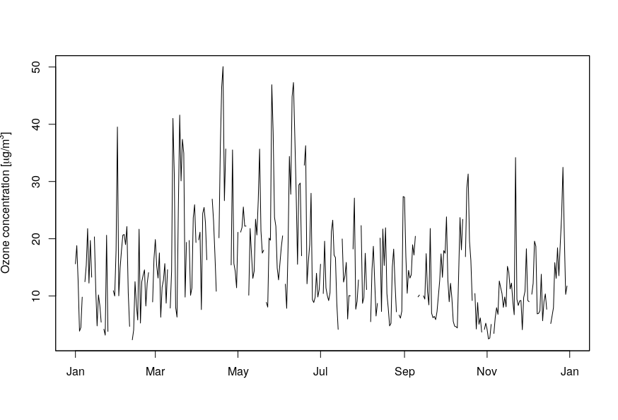

get_hourly_data.png

The above figure shows the highest concentrations happen in late spring and at the beginning of summer. In order to check whether this happens every year, we can download multiple years of data and then compare them.

The code below explores the distribution of ozone by month. The resulting box plots show that the highest concentrations usually occurr during April/May and that these vary year-by-year.

# Get 15 years of hourly ozone data from the same monitoring station
library("ggplot2")
library("dplyr")
library("lubridate")

df <- ukair_get_hourly_data("MY1", years = 2000:2015)

df %>%
  mutate(year = year(datetime),
         month = month(datetime),
         year_month = strftime(datetime, "%Y-%m")) %>%
  group_by(month, year_month) %>%
  summarize(ozone = mean(Ozone, na.rm=TRUE)) %>%
  na.omit %>%
  ggplot() +
  geom_boxplot(aes(x = as.factor(month), y = ozone, group = month),
               outlier.shape = NA) +
  xlab("Month of the year") +
  ylab(expression(paste("Ozone concentration (", mu, "g/",m^3,")"))) +
  ggtitle("15 years of hourly ozone data from London Marylebone Road monitoring station")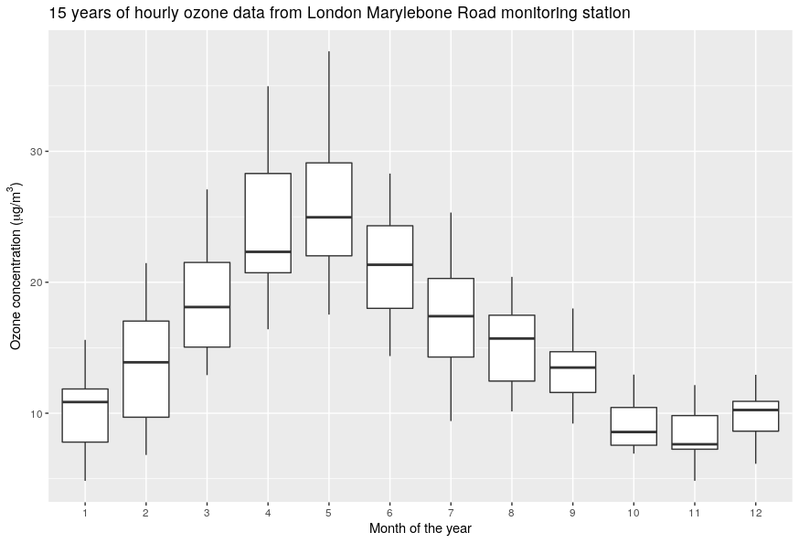

ozone_data.png

Applications

Plotting stations’ locations

After scraping DEFRA’s web pages, almost all the stations have valid coordinates. You can create an interactive map using leaflet. The code below generates a map where blue circles are all the stations with valid coordinates, while red circles show locations with available hourly data.

# Keep only station with coordinates
stations_with_coords <- stations[complete.cases(stations[, c("Longitude",
                                                             "Latitude")]), ]
# Keep only station with known SiteID
stations_with_SiteID <- which(!is.na(stations_with_coords$SiteID))

# An interactive map
library("leaflet")
leaflet(data = stations_with_coords) %>% addTiles() %>% 
  addCircleMarkers(lng = ~Longitude, 
                   lat = ~Latitude,  
                   popup = ~SiteID,
                   radius = 1, color="blue", fill = FALSE) %>%
  addCircleMarkers(lng = ~Longitude[stations_with_SiteID], 
                   lat = ~Latitude[stations_with_SiteID], 
                   radius = 0.5, color="red", 
                   popup = ~SiteID[stations_with_SiteID])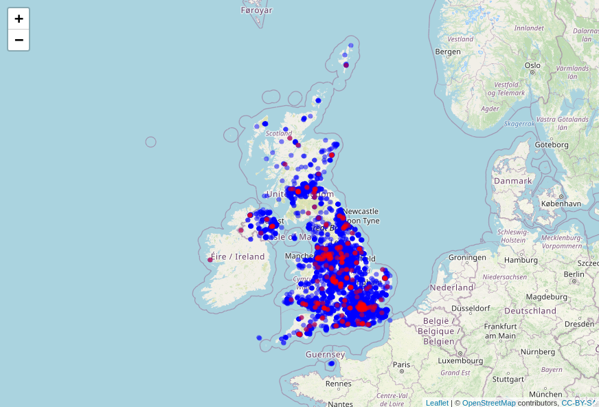

map_data.png

Analyse the spatial distribution of the monitoring stations

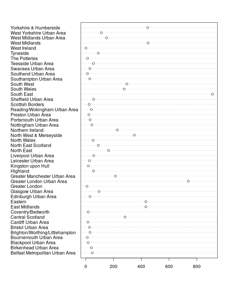
Below are two plots showing the spatial distribution of the monitoring stations. These are concentrated largely in urban areas and mostly estimate the background level of concentration of pollutants.

# Zone
dotchart(as.matrix(table(stations$Zone))[,1])

dotchart_zone.png

# Environment.Type
dotchart(as.matrix(table(stations$Environment.Type[stations$Environment.Type != "Unknown Unknown"]))[,1])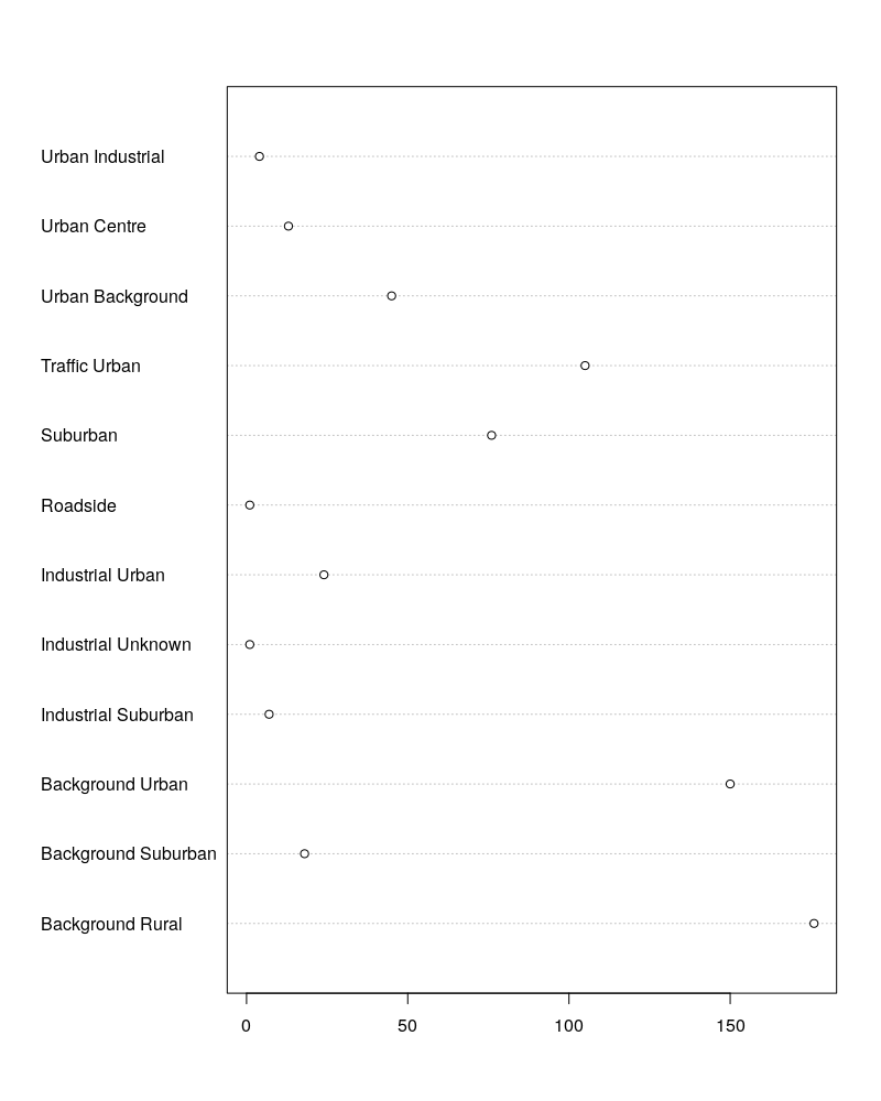

dotchart_envtype.png

Use multiple cores to speed up data retrieval from numerous sites

The acquisition of data from hundreds of sites takes only few minutes:

library("parallel")

# Use detectCores() to find out many cores are available on your machine
cl <- makeCluster(getOption("cl.cores", detectCores()))

system.time(myList <- parLapply(cl, stations$SiteID[stations_with_SiteID], 
                                ukair_get_hourly_data, years=1999:2016))

stopCluster(cl)

df <- bind_rows(myList)

Claudia Vitolo

2022-03-26