Detecting interspecific interactions

Interspecific interactions

Interspecific data can be used with {spatsoc} to estimate interspecific interactions, eg. predator-prey dynamics.

---

See the other vignettes for further information:

• Introduction to spatsoc
  • temporal grouping
  • spatiotemporal grouping with group_pts, group_lines, group_polys
  • distance based edge-list generation with edge_dist
• Frequently asked questions about spatsoc
  • install
  • function details for group_times, group_pts, group_lines, group_polys, edge_dist, edge_nn, and randomizations
  • package design including modify-by-reference, data.table column allocation
  • calculating summary information
• Using spatsoc in social network analysis
  • generating gambit-of-the-group data
  • generating observed networks
  • data stream randomization, randomized networks
  • network metrics
• Using distance based edge-lists generating functions, dyad_id, and fusion_id
  • generate distance based edge-lists with edge_dist and edge_nn
  • generate dyad identifiers for edge-lists with dyad_id
  • identify fusion events with fusion_id
• Geometry interface
  • using get_geometry to setup a geometry column and use the geometry interface
  • details of underlying distance, direction and centroid spatial measures
  • converting to and from related packages
• Interspecific interactions
  • combine two movement datasets
  • identify interspecific interactions

Interspecific interactions

Given two movement datasets, simply bind them together and use the group_* functions as usual.

# Load packages
library(spatsoc)
library(data.table)

# Load data
predator <- fread(system.file("extdata", "DT_predator.csv", package = "spatsoc"))
prey <- fread(system.file("extdata", "DT_prey.csv", package = "spatsoc"))

# Combine data
DT <- rbindlist(list(predator, prey))

# Set the datetime as a POSIxct
DT[, datetime := as.POSIXct(datetime)]


# Temporal grouping
group_times(DT, datetime = 'datetime', threshold = '10 minutes')
#>           ID        X       Y            datetime population     type minutes
#>       <char>    <num>   <num>              <POSc>      <int>   <char>   <int>
#>    1:      B 708315.6 5460839 2016-11-30 14:00:45          1 predator       0
#>    2:      A 709764.2 5458231 2017-01-05 10:00:54          1 predator       0
#>    3:      B 709472.3 5460132 2016-12-03 08:00:42          1 predator       0
#>    4:      A 713630.5 5456393 2017-01-27 02:01:16          1 predator       0
#>    5:      B 707303.2 5461003 2016-12-17 18:00:54          1 predator       0
#>   ---                                                                        
#> 5824:      G 708660.2 5459275 2017-02-28 14:00:44          1     prey       0
#> 5825:      G 708669.4 5459276 2017-02-28 16:00:42          1     prey       0
#> 5826:      G 708212.0 5458998 2017-02-28 18:00:53          1     prey       0
#> 5827:      G 708153.2 5458953 2017-02-28 20:00:12          1     prey       0
#> 5828:      G 708307.6 5459182 2017-02-28 22:00:46          1     prey       0
#>       timegroup
#>           <int>
#>    1:         1
#>    2:         2
#>    3:         3
#>    4:         4
#>    5:         5
#>   ---          
#> 5824:      1422
#> 5825:      1423
#> 5826:      1424
#> 5827:      1425
#> 5828:      1440

# Spatial grouping
group_pts(DT, threshold = 50, id = 'ID', 
          coords = c('X', 'Y'), timegroup = 'timegroup')
#>           ID        X       Y            datetime population     type minutes
#>       <char>    <num>   <num>              <POSc>      <int>   <char>   <int>
#>    1:      B 708315.6 5460839 2016-11-30 14:00:45          1 predator       0
#>    2:      A 709764.2 5458231 2017-01-05 10:00:54          1 predator       0
#>    3:      B 709472.3 5460132 2016-12-03 08:00:42          1 predator       0
#>    4:      A 713630.5 5456393 2017-01-27 02:01:16          1 predator       0
#>    5:      B 707303.2 5461003 2016-12-17 18:00:54          1 predator       0
#>   ---                                                                        
#> 5824:      G 708660.2 5459275 2017-02-28 14:00:44          1     prey       0
#> 5825:      G 708669.4 5459276 2017-02-28 16:00:42          1     prey       0
#> 5826:      G 708212.0 5458998 2017-02-28 18:00:53          1     prey       0
#> 5827:      G 708153.2 5458953 2017-02-28 20:00:12          1     prey       0
#> 5828:      G 708307.6 5459182 2017-02-28 22:00:46          1     prey       0
#>       timegroup group
#>           <int> <int>
#>    1:         1     1
#>    2:         2     2
#>    3:         3     3
#>    4:         4     4
#>    5:         5     5
#>   ---                
#> 5824:      1422  5467
#> 5825:      1423  5468
#> 5826:      1424  5469
#> 5827:      1425  5470
#> 5828:      1440  5471


# Calculate the number of types within each group
DT[, n_type := uniqueN(type), by = group]
DT[, interact := n_type > 1]

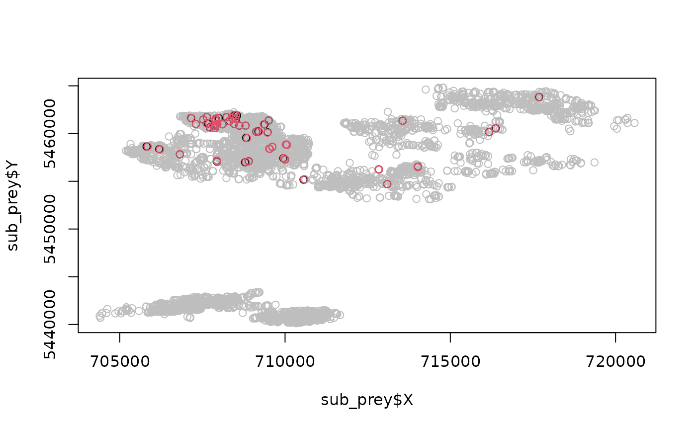
# Prey's perspective
sub_prey <- DT[type == 'prey']
sub_prey[, mean(interact)]
#> [1] 0.01169693


# Plot --------------------------------------------------------------------
# If we subset only where there are interactions
sub_interact <- DT[(interact)]

plot(sub_prey$X, sub_prey$Y, col = 'grey', pch = 21)
points(sub_interact$X, sub_interact$Y, col = factor(sub_interact$type))