Using customized gazetteers
Source:vignettes/Using_custom_gazetteers.Rmd
Using_custom_gazetteers.RmdCoordinateCleaner identifies potentially erroneous geographic records
with coordinates assigned to the sea, countr coordinate, country
capitals, urban areas, institutions, the GBIF headquarters and countries
based on the comparison with geographic gazetteers (i.e. reference
databases). All of these functions include default reference databases
compiled from various sources. These default references have been
selected suitable for regional to global analyses. They will also work
for smaller scale analyses, but in some case different references might
be desirable and available. this could be for instance centroids of
small scale political units, a different set of urban areas, or a
different coastline when working with coastal species. To account for
this, each CoordinateCleaner function using a gazetteer has a
ref argument to specify custom gazetteers.
We will use the case of coastlines and a coastal species to
demonstrate the application of custom gazetteers. The purpose of
cc_sea is to flag records in the sea, since these often
represent erroneous and undesired records for terrestrial organisms. The
standard gazetteer for this function is fetched from
naturalearthdata.com at a 1:50m scale. However, often coordinates
available from public databases are only precise at the scale of
kilometres, which might lead to an overly critical flagging of
coordinates close to the coastline, which is a problem especially for
coastal or intertidal species. WE illustrate the issue on for the
mangrove tree genus Avicennia.
library(CoordinateCleaner)
library(dplyr)
library(ggplot2)
library(rgbif)
library(viridis)
library(terra)

#download data from GBIF
dat <- rgbif::occ_search(scientificName = "Avicennia", limit = 1000,
         hasCoordinate = T)

dat <- dat$data

dat <-  dat %>%
  dplyr::select(species = name, decimalLongitude = decimalLongitude,
         decimalLatitude = decimalLatitude, countryCode)

# run with default gazetteer
outl <- cc_sea(dat, value = "flagged")
## OGR data source with driver: ESRI Shapefile
## Source: "C:\Users\az64mycy\AppData\Local\Temp\Rtmp4SRhHV", layer: "ne_110m_land"
## with 127 features
## It has 3 fields

plo <- data.frame(dat, outlier =  as.factor(!outl))

#plot results
ggplot() +
  borders(fill = "grey60") +
  geom_point(data = plo,
             aes(x = decimalLongitude, y = decimalLatitude, col = outlier)) +
  scale_color_viridis(discrete = T, name = "Flagged outlier") +
  coord_fixed() +
  theme_bw() +
  theme(legend.position = "bottom")
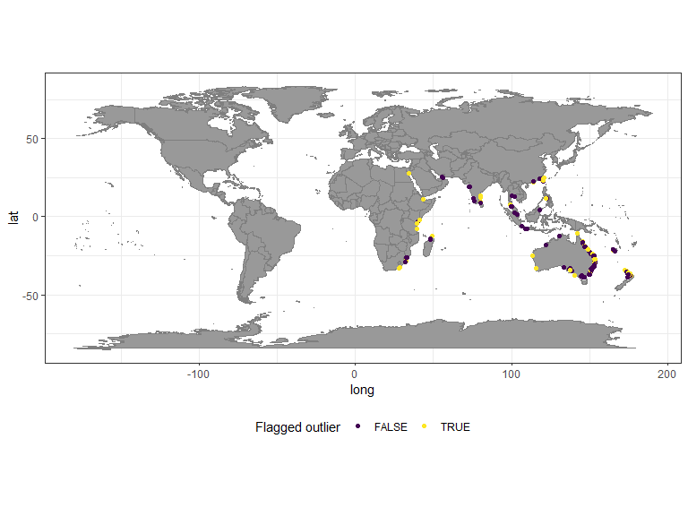
A large number of the coastal records gets flagged, which in this
case is undesirable, because it is not a function of the records being
wrong, but rather of the precision of the coordinates and the resolution
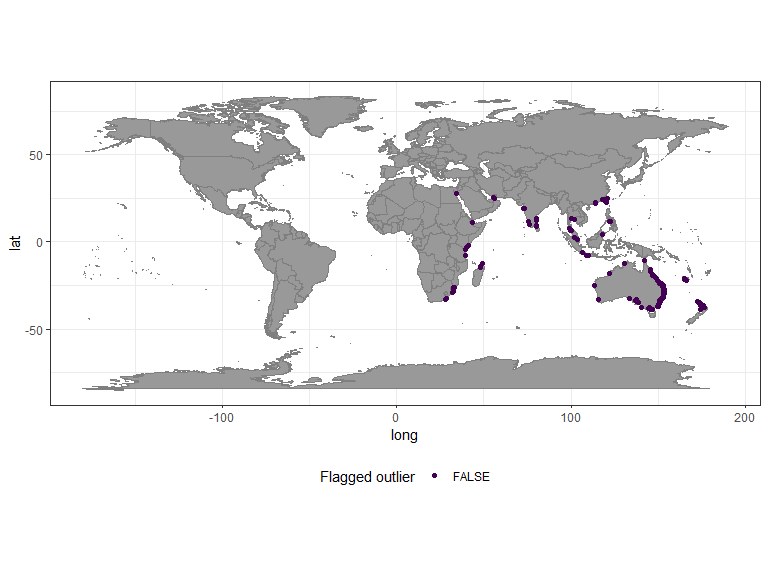
of the reference. To avoid this problem you can use a buffered
reference, which avoids flagging records close to the coast line and
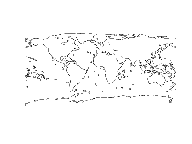
only flags records from the open ocean. CoordinateCleaner comes
with a one degree buffered reference (buffland). In case a
narrower or distance true buffer is necessary, you can provide any
SpatVector similar in structure to buffland via the
ref argument.

# run with custom gazetteer
outl <- cc_sea(dat, value = "flagged", ref = buffland)

plo <- data.frame(dat, outlier =  as.factor(!outl))

#plot results
ggplot()+
  borders(fill = "grey60")+
  geom_point(data = plo,
             aes(x = decimalLongitude, y = decimalLatitude, col = outlier))+
  scale_color_viridis(discrete = T, name = "Flagged outlier")+
  coord_fixed()+
  theme_bw()+
  theme(legend.position = "bottom")