Multicomponent cosinor modeling
Oliver Jayasinghe and Rex Parsons
Source:vignettes/multiple-components.Rmd
multiple-components.RmdGLMMcosinor allows specification of multi-component cosinor models. This is useful if there are multiple explanatory variables with known periods affecting the response variable.
Generating a two-component model
To generate a multi-component model, set n_components in
the amp_acro() part of the formula to the desired number of
components. Then, optionally assign groups to each component in the
group argument. If only one group entry is supplied but
n_components is greater than 1, then the single group entry
will be matched to each component.
The period argument must also match the length of
n_components, where the order of the periods corresponds to
their assigned component. For example, if n_components = 2,
and period = c(12,6), then the first component has a
period of 12 and the second a period of 6. Similarly to the
group argument, if only one period is supplied despite
n_components being greater than 1, then this period will be
matched to each component.
For example:
library(GLMMcosinor)
testdata_two_components <- simulate_cosinor(
  1000,
  n_period = 10,
  mesor = 7,
  amp = c(0.1, 0.4),
  acro = c(1, 1.5),
  beta.mesor = 4.4,
  beta.amp = c(2, 1),
  beta.acro = c(1, -1.5),
  family = "poisson",
  period = c(12, 6),
  n_components = 2,
  beta.group = TRUE
)
object <- cglmm(
  Y ~ group + amp_acro(
    time_col = times,
    n_components = 2,
    period = c(12, 6),
    group = c("group", "group")
  ),
  data = testdata_two_components,
  family = poisson()
)
object
#>
#>  Conditional Model
#>
#>  Raw formula:
#> Y ~ group + group:main_rrr1 + group:main_sss1 + group:main_rrr2 +      group:main_sss2
#>
#>  Raw Coefficients:
#>                  Estimate
#> (Intercept)       6.99894
#> group1           -2.60342
#> group0:main_rrr1  0.05248
#> group1:main_rrr1  1.08250
#> group0:main_sss1  0.08753
#> group1:main_sss1  1.68129
#> group0:main_rrr2  0.02926
#> group1:main_rrr2  0.06860
#> group0:main_sss2  0.40068
#> group1:main_sss2 -0.99822
#>
#>  Transformed Coefficients:
#>                Estimate
#> (Intercept)     6.99894
#> [group=1]      -2.60342
#> [group=0]:amp1  0.10205
#> [group=1]:amp1  1.99964
#> [group=0]:amp2  0.40175
#> [group=1]:amp2  1.00057
#> [group=0]:acr1  1.03070
#> [group=1]:acr1  0.99875
#> [group=0]:acr2  1.49790
#> [group=1]:acr2 -1.50218
In the output, the suffix on the estimates for amplitude and acrophase represents its component:
[group=0]:amp1 = 0.10205represents the estimate for amplitude ofgroup 0for the first component[group=1]:amp1 = 1.99964represents the estimate for amplitude ofgroup 1for the first component[group=0]:amp2 = 0.40175represents the estimate for amplitude ofgroup 0for the second component[group=1]:amp2 = 1.00057represents the estimate for amplitude ofgroup 1for the second componentSimilarly for acrophase estimates
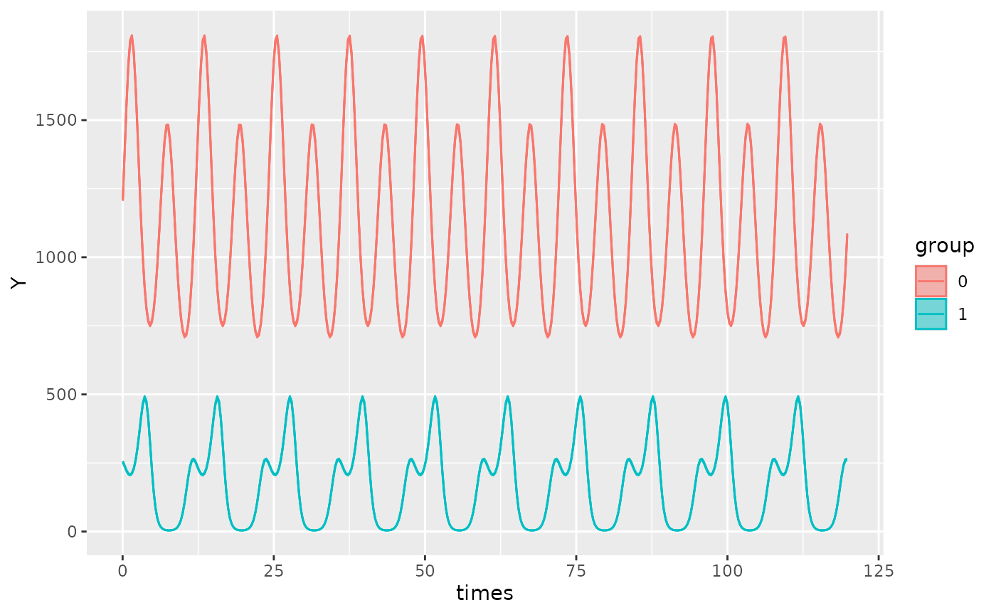
autoplot(object)
If a multicomponent model has one component that is grouped with
other components that aren’t, the vector input for group
must still be the same length as n_components but have the
non-grouped components represented as group = NA.
For example, if wanted only the first component to have a grouped
component, we would specify the group argument as
group = c("group", NA)) . Here, the first component is
grouped by group, and the second component is not grouped.
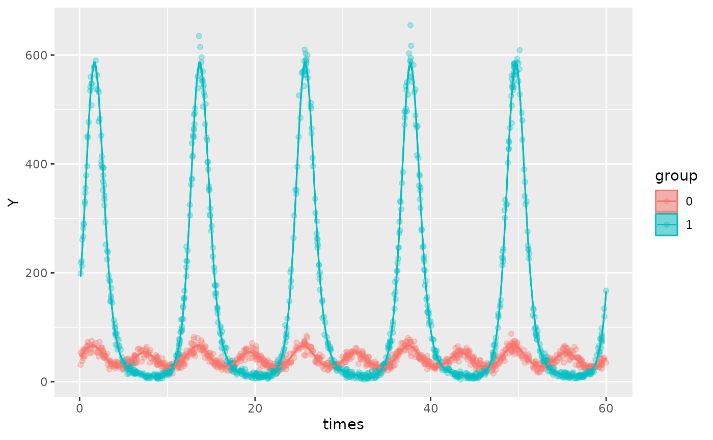
The data was simulated such that the second component was the same for
both groups.
testdata_two_components_grouped <- simulate_cosinor(
  1000,
  n_period = 5,
  mesor = 3.7,
  amp = c(0.1, 0.4),
  acro = c(1, 1.5),
  beta.mesor = 4,
  beta.amp = c(2, 0.4),
  beta.acro = c(1, 1.5),
  family = "poisson",
  period = c(12, 6),
  n_components = 2,
  beta.group = TRUE
)
object <- cglmm(
  Y ~ group + amp_acro(
    time_col = times,
    n_components = 2,
    period = c(12, 6),
    group = c("group", NA)
  ),
  data = testdata_two_components_grouped,
  family = poisson()
)
object
#>
#>  Conditional Model
#>
#>  Raw formula:
#> Y ~ group + main_rrr2 + main_sss2 + group:main_rrr1 + group:main_sss1
#>
#>  Raw Coefficients:
#>                  Estimate
#> (Intercept)       3.69558
#> group1            0.31184
#> main_rrr2         0.02612
#> main_sss2         0.39710
#> group0:main_rrr1  0.04946
#> group1:main_rrr1  1.07681
#> group0:main_sss1  0.09546
#> group1:main_sss1  1.67644
#>
#>  Transformed Coefficients:
#>                Estimate
#> (Intercept)     3.69558
#> [group=1]       0.31184
#> [group=0]:amp1  0.10752
#> [group=1]:amp1  1.99248
#> amp2            0.39795
#> [group=0]:acr1  1.09273
#> [group=1]:acr1  0.99984
#> acr2            1.50512
We would interpret the output the transformed coefficients as follows:
MESOR for
group 0is3.69558.MESOR difference to
group 0forgroup 1is[group=1] = 0.31184The estimate for the amplitude of the first component for
group 0is[group=0]:amp1 = 0.10752The estimate for the amplitude of the first component for
group 1is[group=1]:amp1 = 1.99248The estimate for the amplitude of the second component is
amp2 = 0.39795and the same for bothgroup 0andgroup 1The estimate for the acrophase of the first component for
group 0is[group=0]:acr1 = 1.09273radiansThe estimate for the acrophase of the first component for
group 1is[group=1]:acr1 = 0.99984radiansThe estimate for the acrophase of the second component is
acr2 = 1.50512radians and is the same for bothgroup 0andgroup 1
autoplot(object, superimpose.data = TRUE)
In this example, it is not strictly necessary to specify
group = c("group", NA)) since specifying
group = c("group","group")still yields accurate
estimates:
object <- cglmm(
  Y ~ group + amp_acro(
    time_col = times,
    n_components = 2,
    period = c(12, 6),
    group = c("group", "group")
  ),
  data = testdata_two_components_grouped,
  family = poisson()
)
object
#>
#>  Conditional Model
#>
#>  Raw formula:
#> Y ~ group + group:main_rrr1 + group:main_sss1 + group:main_rrr2 +      group:main_sss2
#>
#>  Raw Coefficients:
#>                  Estimate
#> (Intercept)       3.69549
#> group1            0.31048
#> group0:main_rrr1  0.05027
#> group1:main_rrr1  1.07082
#> group0:main_sss1  0.09515
#> group1:main_sss1  1.68461
#> group0:main_rrr2  0.01368
#> group1:main_rrr2  0.03613
#> group0:main_sss2  0.39617
#> group1:main_sss2  0.39776
#>
#>  Transformed Coefficients:
#>                Estimate
#> (Intercept)     3.69549
#> [group=1]       0.31048
#> [group=0]:amp1  0.10761
#> [group=1]:amp1  1.99614
#> [group=0]:amp2  0.39641
#> [group=1]:amp2  0.39939
#> [group=0]:acr1  1.08472
#> [group=1]:acr1  1.00457
#> [group=0]:acr2  1.53629
#> [group=1]:acr2  1.48022
If a multicomponent model is specified
(n_components > 1) but the length of group
or period is 1, then it will be assumed that the one
group and/or period values specified apply to
all components. For example, if n_components = 2 ,
but group = "group", then the one element in this
group vector will be replicated to produce
group = c("group","group")which now has a length that
matches n_components. The same applies for
period.
For instance, the following two cglmm() calls fit the
same models:
cglmm(
  Y ~ group + amp_acro(times,
    n_components = 2,
    period = 12,
    group = "group"
  ),
  data = testdata_two_components,
  family = poisson()
)
#>
#>  Conditional Model
#>
#>  Raw formula:
#> Y ~ group + group:main_rrr1 + group:main_sss1
#>
#>  Raw Coefficients:
#>                  Estimate
#> (Intercept)       7.04448
#> group1           -2.22027
#> group0:main_rrr1  0.07222
#> group1:main_rrr1  0.39492
#> group0:main_sss1  0.11292
#> group1:main_sss1  1.11176
#>
#>  Transformed Coefficients:
#>                Estimate
#> (Intercept)     7.04448
#> [group=1]      -2.22027
#> [group=0]:amp1  0.13404
#> [group=1]:amp1  1.17982
#> [group=0]:amp2  0.13404
#> [group=1]:amp2  1.17982
#> [group=0]:acr1  1.00181
#> [group=1]:acr1  1.22947
#> [group=0]:acr2  1.00181
#> [group=1]:acr2  1.22947


cglmm(
  Y ~ group + amp_acro(times,
    n_components = 2,
    period = c(12, 12),
    group = c("group", "group")
  ),
  data = testdata_two_components,
  family = poisson()
)
#>
#>  Conditional Model
#>
#>  Raw formula:
#> Y ~ group + group:main_rrr1 + group:main_sss1
#>
#>  Raw Coefficients:
#>                  Estimate
#> (Intercept)       7.04448
#> group1           -2.22027
#> group0:main_rrr1  0.07222
#> group1:main_rrr1  0.39492
#> group0:main_sss1  0.11292
#> group1:main_sss1  1.11176
#>
#>  Transformed Coefficients:
#>                Estimate
#> (Intercept)     7.04448
#> [group=1]      -2.22027
#> [group=0]:amp1  0.13404
#> [group=1]:amp1  1.17982
#> [group=0]:amp2  0.13404
#> [group=1]:amp2  1.17982
#> [group=0]:acr1  1.00181
#> [group=1]:acr1  1.22947
#> [group=0]:acr2  1.00181
#> [group=1]:acr2  1.22947
Generating a three-component model
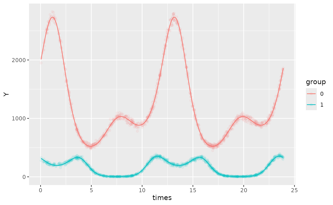
The plot below shows a 3-component model with the simulated data overlayed:
testdata_three_components <- simulate_cosinor(
  1000,
  n_period = 2,
  mesor = 7,
  amp = c(0.1, 0.4, 0.5),
  acro = c(1, 1.5, 0.1),
  beta.mesor = 4.4,
  beta.amp = c(2, 1, 0.4),
  beta.acro = c(1, -1.5, -1),
  family = "poisson",
  period = c(12, 6, 12),
  n_components = 3,
  beta.group = TRUE
)
object <- cglmm(
  Y ~ group + amp_acro(times,
    n_components = 3,
    period = c(12, 6, 12),
    group = "group"
  ),
  data = testdata_three_components,
  family = poisson()
)
autoplot(object,
  superimpose.data = TRUE,
  x_str = "group",
  predict.ribbon = FALSE,
  data_opacity = 0.08
)