Installation
Install the development version of allodb from GitHub:
# install.packages("pak")
pak::pak("ropensci/allodb")
Load the census data
Prior to calculating tree biomass using allodb, users need to provide a table (i.e. dataframe) with DBH (cm), parsed species Latin names, and site(s) coordinates. In the following examples we use data from the Smithsonian Conservation Biology Institute, USA (SCBI) ForestGEO dynamics plot (1st census in 2008, trees from 1 hectare). Data can be requested through the ForestGEO portal (https://forestgeo.si.edu/)
require(allodb)
#> Loading required package: allodb
data(scbi_stem1)
str(scbi_stem1)
#> Classes 'tbl_df', 'tbl' and 'data.frame':    2287 obs. of  6 variables:
#>  $ treeID : int  2695 1229 1230 1295 1229 66 2600 4936 1229 1005 ...
#>  $ stemID : int  2695 38557 1230 32303 32273 31258 2600 4936 36996 1005 ...
#>  $ dbh    : num  1.41 1.67 1.42 1.04 2.47 ...
#>  $ genus  : chr  "Acer" "Acer" "Acer" "Acer" ...
#>  $ species: chr  "negundo" "negundo" "negundo" "negundo" ...
#>  $ Family : chr  "Sapindaceae" "Sapindaceae" "Sapindaceae" "Sapindaceae" ...
Load and modify the equation table
allodb provides a dataframe containing 570 parsed
allometric equations.
data(equations)Additional information about the equation table can be found in the equation metadata.
data(equations_metadata)This equation table is the default in all functions of the package.
Users can modify the set of equations that will be used to estimate
biomass using the new_equations() function: users can work
on a subset of those equations, or add new equations to the table (see
?allodb::new_equations). The customized equation table
should be provided as an argument in the get_biomass() (or
other) function (argument name: new_eqtable).
Subset the equation table
show_cols <- c("equation_id", "equation_taxa", "equation_allometry")
eq_tab_acer <- new_equations(subset_taxa = "Acer")
head(eq_tab_acer[, show_cols])
#> # A tibble: 6 × 3
#>   equation_id equation_taxa       equation_allometry
#>   <chr>       <chr>               <chr>
#> 1 a4e4d1      Acer saccharum      exp(-2.192-0.011*dbh+2.67*(log(dbh)))
#> 2 dfc2c7      Acer rubrum         2.02338*(dbh^2)^1.27612
#> 3 eac63e      Acer rubrum         5.2879*(dbh^2)^1.07581
#> 4 f49bcb      Acer pseudoplatanus exp(-5.644074+(2.5189*(log(pi*dbh))))
#> 5 14bf3d      Acer mandshuricum   0.0335*(dbh)^1.606+0.0026*(dbh)^3.323+0.1222*…
#> 6 0c7cd6      Acer mono           0.0202*(dbh)^1.810+0.0111*(dbh)^2.740+0.1156*…
Add new equations
eq_tab_add <- new_equations(
  new_taxa = c("Quercus ilex", "Castanea sativa"),
  new_allometry = c("0.12*dbh^2.5", "0.15*dbh^2.7"),
  new_coords = c(4, 44),
  new_min_dbh = c(5, 10),
  new_max_dbh = c(35, 68),
  new_sample_size = c(143, 62)
)
## show added equations - they contain "new" in their equation_id
head(eq_tab_add[grepl("new", eq_tab_add$equation_id), ])
#> # A tibble: 2 × 15
#>   equation_id equation_taxa   equation_allometry independent_variable
#>   <chr>       <chr>           <chr>              <chr>
#> 1 new1        Quercus ilex    0.12*dbh^2.5       DBH
#> 2 new2        Castanea sativa 0.15*dbh^2.7       DBH
#> # ℹ 11 more variables: dependent_variable <chr>, long <chr>, lat <chr>,
#> #   koppen <chr>, dbh_min_cm <dbl>, dbh_max_cm <dbl>, sample_size <dbl>,
#> #   dbh_units_original <chr>, dbh_unit_cf <dbl>, output_units_original <chr>,
#> #   output_units_cf <dbl>
Estimate the aboveground biomass
The aboveground biomass (AGB) can be estimated using the
get_biomass() function: the required arguments are the
diameter at breast height (DBH, in cm), the taxonomic identification (to
the genus or species level), and the location (long-lat coordinates).
The output is the aboveground biomass of the tree in kg.
get_biomass(
dbh = 50,
genus = "liriodendron",
species = "tulipifera",
coords = c(-78.2, 38.9)
)
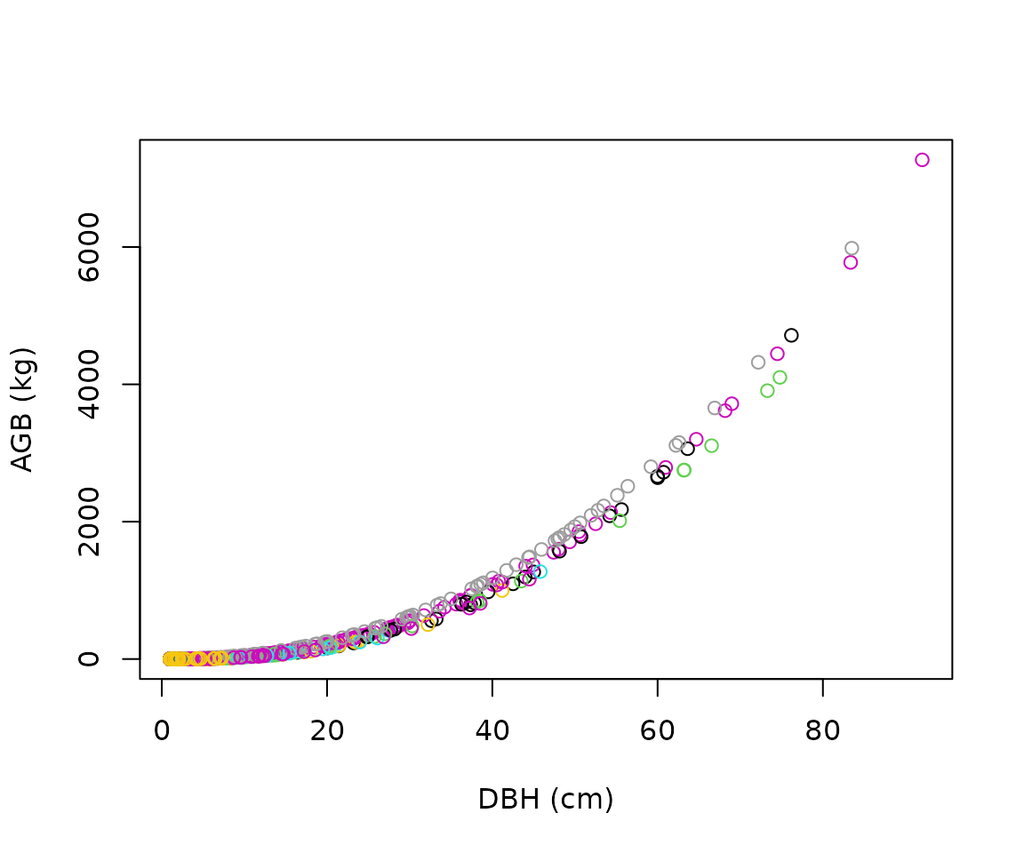
#> [1] 1578.644The get_biomass() function can also be used to estimate
the AGB of all trees in one (or several) censuses.
scbi_stem1$agb <-
  get_biomass(
    dbh = scbi_stem1$dbh,
    genus = scbi_stem1$genus,
    species = scbi_stem1$species,
    coords = c(-78.2, 38.9)
  )
plot(
  x = scbi_stem1$dbh,
  y = scbi_stem1$agb,
  col = factor(scbi_stem1$genus),
  xlab = "DBH (cm)",
  ylab = "AGB (kg)"
)
How AGB is estimated
Attribute a weight to each equation in the equation table for each taxon/location combination
Within the get_biomass() function, new allometric
equations are calibrated for each taxon/location combinations in the
user-provided dataframe. This is done by attributing a weight to each
equation in the equation table, based on its sampling size, and
taxonomic and climatic similarity with the taxon/location combination
considered.
allom_weights <-
weight_allom(
genus = "Acer",
species = "rubrum",
coords = c(-78, 38)
)
## visualize weights
equ_tab_acer <- new_equations()
equ_tab_acer$weights <- allom_weights
keep_cols <-
c(
"equation_id",
"equation_taxa",
"sample_size",
"weights"
)
order_weights <- order(equ_tab_acer$weights, decreasing = TRUE)
equ_tab_acer <- equ_tab_acer[order_weights, keep_cols]
head(equ_tab_acer)
#> # A tibble: 6 × 4
#> equation_id equation_taxa sample_size weights
#> <chr> <chr> <dbl> <dbl>
#> 1 138258 Acer rubrum 150 0.415
#> 2 d6be5c Sapindaceae 243 0.383
#> 3 a2fbbb Sapindaceae 200 0.349
#> 4 2630d5 Trees (Angiosperms) 886 0.299
#> 5 d4c590 Trees (Angiosperms) 549 0.289
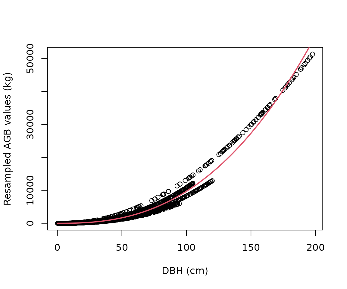
#> 6 ed748f Broad-leaved species 2223 0.270Resample equations
Equations are then resampled within their original DBH range: the
number of resampled values for each equation is proportional to its
weight (as attributed by the weight_allom() function).
df_resample <-
  resample_agb(
    genus = "Acer",
    species = "rubrum",
    coords = c(-78, 38),
    nres = 1e4
  )

plot(
  df_resample$dbh,
  df_resample$agb,
  xlab = "DBH (cm)",
  ylab = "Resampled AGB values (kg)"
)
Calibrate a new equation for each taxon/location combination
The resampled values are then used to fit the following nonlinear
model:
,
with i.i.d.
.
The parameters (a, b, and sigma) are returned
by the est_params() function. In other words, this function
calibrates new allometric equations from sampling previous ones. New
allometric equations are calibrated for each species and location by
resampling the original compiled equations; equations with a larger
sample size, and/or higher taxonomic rank, and climatic similarity with
the species and location in question are given a higher weight in this
process.
pars_acer <- est_params(
  genus = "Acer",
  species = "rubrum",
  coords = c(-78, 38)
)
plot(
  df_resample$dbh,
  df_resample$agb,
  xlab = "DBH (cm)",
  ylab = "Resampled AGB values (kg)"
)
curve(pars_acer$a * x^pars_acer$b,
  add = TRUE, col = 2, lwd = 2
)
The est_params() function can be used for all
species/site combinations in the dataset at once.
params <- est_params(
  genus = scbi_stem1$genus,
  species = scbi_stem1$species,
  coords = c(-78.2, 38.9)
)
head(params)
#> # A tibble: 6 × 7
#>   genus       species      long   lat      a     b sigma
#>   <chr>       <chr>       <dbl> <dbl>  <dbl> <dbl> <dbl>
#> 1 Acer        negundo     -78.2  38.9 0.0762  2.55  433.
#> 2 Acer        rubrum      -78.2  38.9 0.0768  2.55  412.
#> 3 Ailanthus   altissima   -78.2  38.9 0.0995  2.48  377.
#> 4 Amelanchier arborea     -78.2  38.9 0.0690  2.56  359.
#> 5 Asimina     triloba     -78.2  38.9 0.0995  2.48  377.
#> 6 Carpinus    caroliniana -78.2  38.9 0.0984  2.48  317.
AGB is then recalculated as AGB = a * dbh^b within the
get_biomass() function.
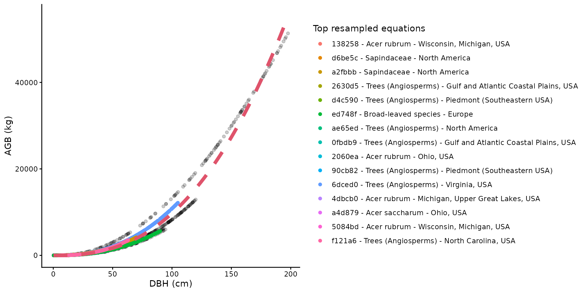
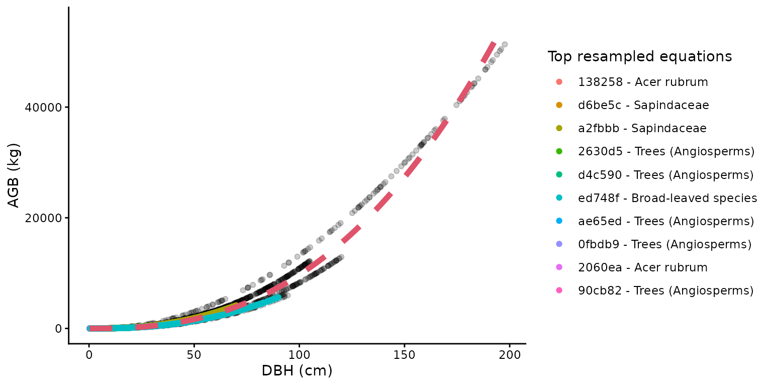
Visualize the recalibration of equations
The recalibrated equation for one taxon/location combination can be
easily visualized with the illustrate_allodb() function,
which returns a ggplot (see package ggplot2) with all
resampled values, and the top equations used displayed in the legend.
The user can control the number of equations and equation information
shown in the legend. The red dotted line is the recalibrated equation
used in the get_biomass() function.
illustrate_allodb(
  genus = "Acer",
  species = "rubrum",
  coords = c(-78, 38)
)
illustrate_allodb(
  genus = "Acer",
  species = "rubrum",
  coords = c(-78, 38),
  neq = 15,
  eqinfo = c("equation_taxa", "geographic_area")
)