Nested Sampling

Richèl J.C. Bilderbeek

2024-11-24

Introduction

This vignette demonstrates how to use the Nested Sampling approach to obtain the marginal likelihood and a Bayes factor, as described in [1]

Setup

library(babette)
#> Loading required package: beautier
#> Loading required package: beastier
#> 
#> Attaching package: 'beastier'
#> The following objects are masked from 'package:beautier':
#> 
#>     is_on_appveyor, is_on_ci, is_on_travis
#> Loading required package: mauricer
#> Warning: package 'mauricer' was built under R version 4.4.2
#> Loading required package: tracerer

babette needs to have ‘BEAST2’ installed to work.

In the case ‘BEAST2’ is not installed, we’ll use this fabricated data:

out_jc69 <- create_test_bbt_run_output()
out_jc69$ns$marg_log_lik <- c(-1.1)
out_jc69$ns$marg_log_lik_sd <- c(0.1)
out_gtr <- out_jc69

Here we setup how to interpret the Bayes factor:

interpret_bayes_factor <- function(bayes_factor) {
  if (bayes_factor < 10^-2.0) {
    "decisive for GTR"
  } else if (bayes_factor < 10^-1.5) {
    "very strong for GTR"
  } else if (bayes_factor < 10^-1.0) {
    "strong for GTR"
  } else if (bayes_factor < 10^-0.5) {
    "substantial for GTR"
  } else if (bayes_factor < 10^0.0) {
    "barely worth mentioning for GTR"
  } else if (bayes_factor < 10^0.5) {
    "barely worth mentioning for JC69"
  } else if (bayes_factor < 10^1.0) {
    "substantial for JC69"
  } else if (bayes_factor < 10^1.5) {
    "strong for JC69"
  } else if (bayes_factor < 10^2.0) {
    "very strong for JC69"
  } else {
    "decisive for JC69"
  }
}
# Should all be TRUE
interpret_bayes_factor(1 / 123.0) == "decisive for GTR"
#> [1] TRUE
interpret_bayes_factor(1 / 85.0) == "very strong for GTR"
#> [1] TRUE
interpret_bayes_factor(1 / 12.5) == "strong for GTR"
#> [1] TRUE
interpret_bayes_factor(1 / 8.5) == "substantial for GTR"
#> [1] TRUE
interpret_bayes_factor(1 / 1.5) == "barely worth mentioning for GTR"
#> [1] TRUE
interpret_bayes_factor(0.99) == "barely worth mentioning for GTR"
#> [1] TRUE
interpret_bayes_factor(1.01) == "barely worth mentioning for JC69"
#> [1] TRUE
interpret_bayes_factor(1.5) == "barely worth mentioning for JC69"
#> [1] TRUE
interpret_bayes_factor(8.5) == "substantial for JC69"
#> [1] TRUE
interpret_bayes_factor(12.5) == "strong for JC69"
#> [1] TRUE
interpret_bayes_factor(85.0) == "very strong for JC69"
#> [1] TRUE
interpret_bayes_factor(123.0) == "decisive for JC69"
#> [1] TRUE

Experiment

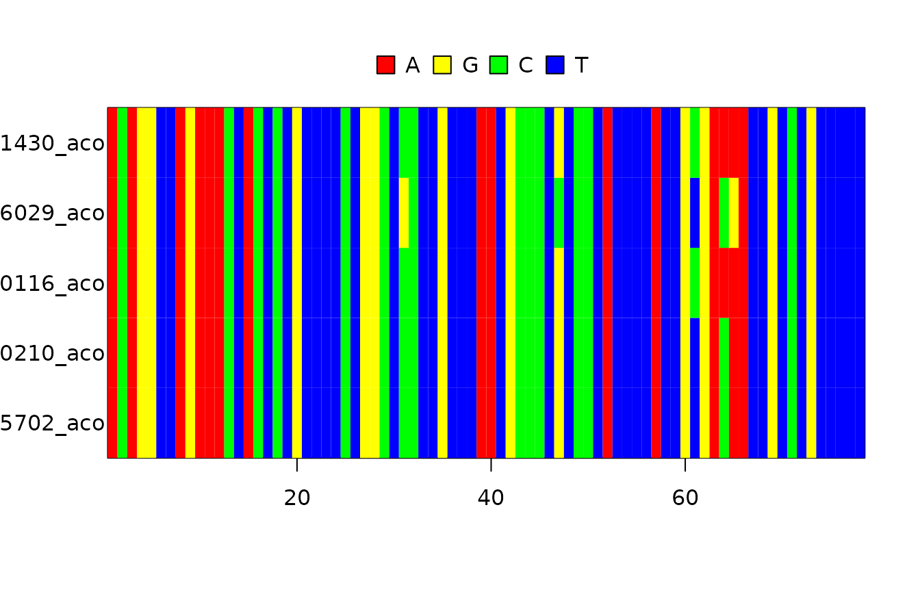
In this experiment, we will use the same DNA alignment to see which DNA nucleotide substitution model is the better fit.

Load the DNA alignment, a subset of taxa from [2]:

fasta_filename <- get_babette_path("anthus_aco_sub.fas")
image(ape::read.FASTA(fasta_filename))

Do the run

In this vignette, the MCMC run is set up to be short:

mcmc <- beautier::create_test_ns_mcmc()

For academic research, better use a longer MCMC chain (with an effective sample size above 200).

Here we do two ‘BEAST2’ runs, with both site models:

if (is_beast2_installed() && is_beast2_pkg_installed("NS")) {
  inference_model <- create_inference_model(
    site_model = beautier::create_jc69_site_model(),
    mcmc = mcmc
  )
  beast2_options <- create_beast2_options(
    beast2_path = beastier::get_default_beast2_bin_path()
  )
  out_jc69 <- bbt_run_from_model(
    fasta_filename = fasta_filename,
    inference_model = inference_model,
    beast2_options = beast2_options
  )
  bbt_delete_temp_files(
    inference_model = inference_model,
    beast2_options = beast2_options
  )
  inference_model <- create_inference_model(
    site_model = beautier::create_gtr_site_model(),
    mcmc = mcmc
  )
  beast2_options <- create_beast2_options(
    beast2_path = beastier::get_default_beast2_bin_path()
  )
  out_gtr <- bbt_run_from_model(
    fasta_filename = fasta_filename,
    inference_model = inference_model,
    beast2_options = beast2_options
  )
  bbt_delete_temp_files(
    inference_model = inference_model,
    beast2_options = beast2_options
  )
}

I will display the marginal likelihoods in a nice table:

if (is_beast2_installed() && is_beast2_pkg_installed("NS")) {
  df <- data.frame(
    model = c("JC69", "GTR"),
    mar_log_lik = c(out_jc69$ns$marg_log_lik, out_gtr$ns$marg_log_lik),
    mar_log_lik_sd = c(out_jc69$ns$marg_log_lik_sd, out_gtr$ns$marg_log_lik_sd)
  )
  knitr::kable(df)
}

The Bayes factor is ratio between the marginal (non-log) likelihoods. In this case, we use the simpler JC69 model as a focus:

if (is_beast2_installed() && is_beast2_pkg_installed("NS")) {
  bayes_factor <- exp(out_jc69$ns$marg_log_lik) / exp(out_gtr$ns$marg_log_lik)
  print(interpret_bayes_factor(bayes_factor))
}

Whatever the support is, be sure to take the error of the marginal likelihood estimation into account.

References

• [1] Maturana, P., Brewer, B. J., Klaere, S., & Bouckaert, R. (2017). Model selection and parameter inference in phylogenetics using Nested Sampling. arXiv preprint arXiv:1703.05471.
• [2] Van Els, Paul, and Heraldo V. Norambuena. “A revision of species limits in Neotropical pipits Anthus based on multilocus genetic and vocal data.” Ibis.