Introduction to concstats

The goal of the concstats package is to offer a set of alternative and/or additional measures to better determine a given market structure and therefore reduce uncertainty with respect to a given market situation. Various functions or groups of functions are available to achieve the desired goal.

Installation

You can install concstats directly from CRAN or the latest development version from github (requires remotes or devtools) remotes::install_github(“ropensci/concstats”)

Then, load the package.

library(concstats)

Data

The following examples use mainly fictitious data to present the functions. However, if you want to test the functionality in more detail, the package comes with a small data set of real Paraguayan credit cooperatives (creditcoops). There are 22 paired observations for real Paraguayan credit cooperatives (with assets > 11 Mio. USD) for 2016 and 2018 with their respective total loans granted. For a better visualization there is an additional column with the transformed total loans. For further information on the data please see the creditcoops help file. For a practical implementation you might be interested to read the following article.

data("creditcoops")
head(creditcoops)
#>   coop_id year total_loans paired total_loans_log
#> 1       1 2016   173892358      1        18.97395
#> 2       1 2018   199048199      1        19.10906
#> 3       2 2016   323892456      2        19.59592
#> 4       2 2018   461609439      2        19.95023
#> 5       3 2016   179981404      3        19.00836
#> 6       3 2018   227232008      3        19.24148

Group wrapper overview

At the moment, there are the following groups of functions available:
- concstats_mstruct() is a wrapper for market structure measures
- concstats_inequ() is a wrapper for inequality and diversity measures
- concstats_comp() is a wrapper with different concentration measures
- concstats_concstats() is a function which calculates a set of pre-selected measures in a one step procedure to get a quick overview of a given market structure

The functions will be presented in more details in the following short step-by-step guide.

Examples

We will use a vector which represents market participants with their respective market shares (in decimal form):

concstats_mstruct

The wrapper includes the following arguments to calculate individual functions: firm, nrs_eq, top, top3, top5, and all. You can also pass the additional argument digits to all, which controls for the number of digits to be printed.
All individual functions can be accessed directly with the prefix “concstats_” (e.g. “concstats_firm” or “concstats_all_mstruct”). The concstats_top_df functions also take a data frame as input, since the ranking of firms might be of interest.

x <- c(0.35, 0.4, 0.05, 0.1, 0.06, 0.04, 0, 0)
test_firm <- concstats_firm(x) # number of firms
test_firm
#> [1] 6

You should have noticed that the market shares are in decimal form. However, you can use integers or floating point numeric types to express market shares. All concstats functions will take care of this and convert theses vectors into decimal form. There are eight market participants, however, two have no market shares, by default concstats treats 0 as NA. The result is a cumulative top 5 market share of 96 %.
You can also access each function through their respective argument in the group wrapper:

x <- c(0.35, 0.4, 0.05, 0.1, 0.06, 0.04, 0, 0)
test_share_top3 <- concstats_mstruct(x, type = "top3") # top3 market shares in %
test_share_top3
#> [1] 85

x <- c(0.35, 0.4, 0.05, 0.1, 0.06, 0.04)
id <- c("firm1", "firm2", "firm3", "firm4", "firm5", "firm6")
test_df <- data.frame(id, x)
concstats_top3_df(test_df, "x")
#>      id    x
#> 2 firm2 0.40
#> 1 firm1 0.35
#> 4 firm4 0.10

Or, just calculate all measures of the group wrapper, and store it in a named object.

x <- c(0.35, 0.4, 0.05, 0.1, 0.06, 0.04, 0, 0)
concstats_all_mstruct(x, na.rm = TRUE, digits = 3)
#>          Measure Value
#> 1          Firms  6.00
#> 2 Nrs_equivalent  3.33
#> 3        Top (%) 40.00
#> 4       Top3 (%) 85.00
#> 5       Top5 (%) 96.00

The result is a data frame of market structure measures.

concstats_inequ

The inequality and diversity group has the following arguments: entropy, gini, simpson, palma, grs, and all. They can also be accessed as individual functions.

x <- c(0.35, 0.4, 0.05, 0.1, 0.06, 0.04)
test_share_entropy <- concstats_entropy(x)
test_share_entropy
#> [1] 0.787806

# and as a non-normalized value
test_share_entropy2 <- concstats_entropy(x, normalized = FALSE)
test_share_entropy2
#> [1] 2.036449

concstats_comp

The group wrapper for competition measures includes the following arguments to calculate hhi, hhi_d, hhi_min, dom, sten, and all.

x <- c(0.35, 0.4, 0.05, 0.1, 0.06, 0.04, 0, 0)
test_share_hhi <- concstats_hhi(x)
test_share_hhi
#> [1] 0.3002

# a normalized value
test_share_hhi2 <- concstats_hhi(x, normalized = TRUE)
test_share_hhi2
#> [1] 0.16024

# the min average of the hhi
test_share_hhi3 <- concstats_comp(x, type = "hhi_min")
test_share_hhi3
#> [1] 0.1666667

concstats_concstats

A single function which calculates a set of eight pre-selected measures in a one step procedure for a first overview of a given market structure. The resulting data frame contains eight measures, which are: number of firms with market share, numbers equivalent, the cumulative share of the top (top 3 and top 5) firm(s) in percentage, the hhi index, the entropy index, and the palma ratio.

x<- c(0.2, 0.3, 0.5)
test_share_conc <- concstats_concstats(x, digit = 2)
test_share_conc
#>          Measure  Value
#> 1          Firms   3.00
#> 2 Nrs_equivalent   2.63
#> 3        Top (%)  50.00
#> 4       Top3 (%) 100.00
#> 5       Top5 (%) 100.00
#> 6            HHI   0.38
#> 7        Entropy   0.94
#> 8    Palma ratio   2.50

Visualization

The scope of the package is to calculate market structure and concentration measures to get a quick and more informed overview of a given market situation. However, it is good practice to visualize your data in an exploratory step or in reporting your results. The package concstats works fine with other Exploratory Data Analysis (EDA) packages or data visualization packages e.g. overviewR, dataexplorer, kableExtra or ggplot2 to name a few.

Some examples on how you can accomplish this. Let us assume one would like to use the group measure for e.g. market structure, and keep the resulting data frame. We can refine the table using kableExtra which works nice with knitr.

This time, we will use our creditcoops data set again, which comes with the package.

data("creditcoops")
head(creditcoops)
#>   coop_id year total_loans paired total_loans_log
#> 1       1 2016   173892358      1        18.97395
#> 2       1 2018   199048199      1        19.10906
#> 3       2 2016   323892456      2        19.59592
#> 4       2 2018   461609439      2        19.95023
#> 5       3 2016   179981404      3        19.00836
#> 6       3 2018   227232008      3        19.24148

You will need the following two packages. Make sure you have these packages installed.

library(dplyr)
library(kableExtra)

Now, we will filter out data for the year 2016.

coops_2016 <- creditcoops %>% dplyr::filter(year == 2016)
head(coops_2016)

coops_2016 <- coops_2016[["total_loans"]] # atomic vector of total loans
coops_2016 <- coops_2016 / sum(coops_2016)  # market shares in decimal form

# We then use the new object `coops_2016` to calculate the market structure
# measures as a group in a one-step-procedure and capture the results in a
# printed table:
coops_2016_mstruct <- concstats_mstruct(coops_2016, type = "all", digits = 2)
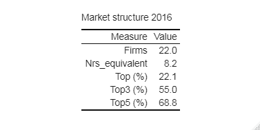
coops_2016_mstruct_tab <- coops_2016_mstruct %>%
  kableExtra::kbl(caption = "Market structure 2016", digits = 2,
                  booktabs = TRUE, align = "r") %>%
  kableExtra::kable_classic(full_width = FALSE, html_font = "Arial")
coops_2016_mstruct_tab

The result is a nice reusable table.

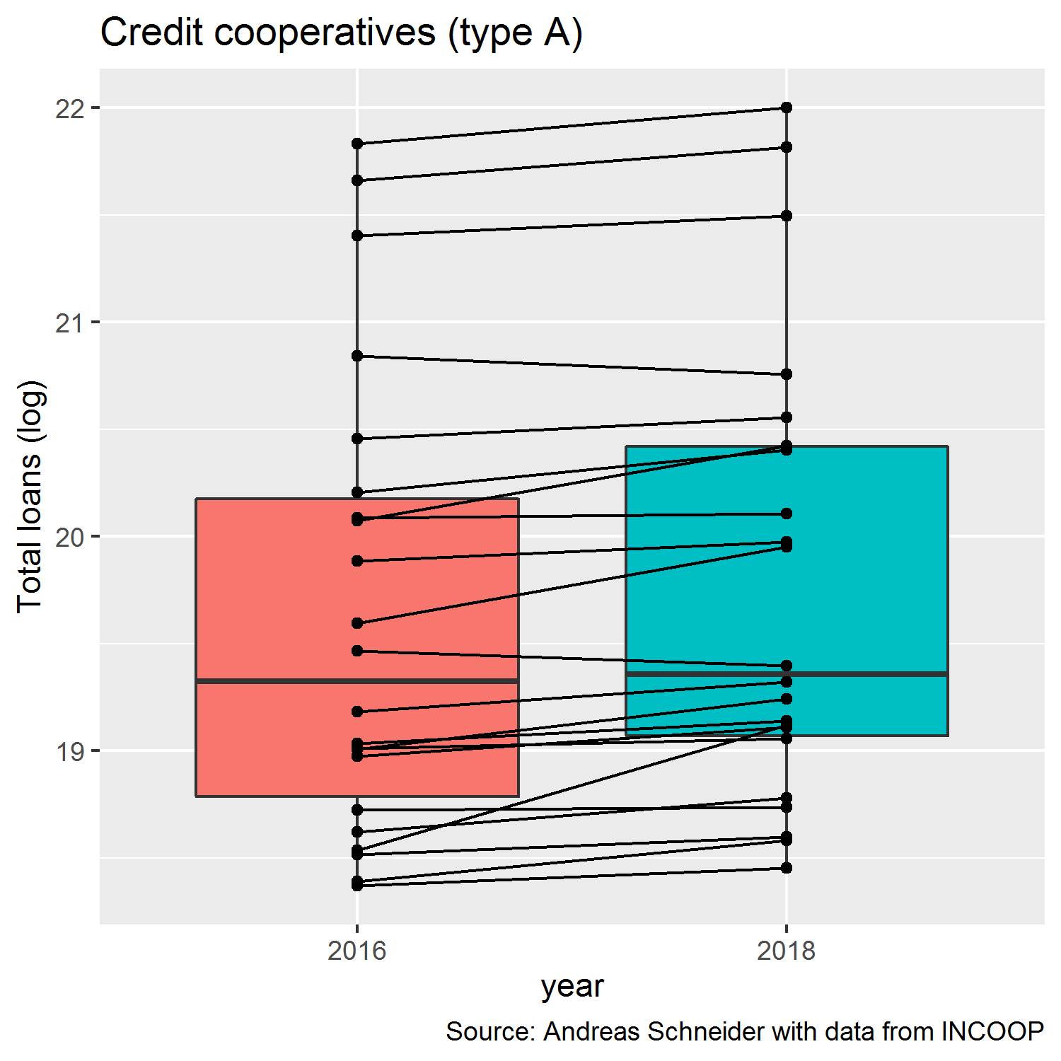
Now, let’s go a step further. We will compare the two samples for 2016 and 2018. For this purpose, we will select from our creditcoops data set the relevant columns (coop_id, year, paired, and total_loans_log) and make a new data frame.

Make sure you have the ggplot2 package installed. Load the package.

library(ggplot2) # Data Visualizations Using the Grammar of Graphics

df_shares_plot <- df_shares %>%
  ggplot(aes(year, total_loans_log, fill = year)) +
  geom_boxplot() +
  geom_point() +
  geom_line(aes(group = paired)) +
  labs(title = "Credit cooperatives (type A)", y = "Total loans (log)",
       caption = "Source: Andreas Schneider with data from INCOOP") +
  theme(legend.position = "none")
df_shares_plot

Having a look a the output, we see a box plot with paired values of the cooperatives and the evolution of their respective total loans over time for the two sample years 2016 and 2018. It seems that most of the cooperatives have increased their amounts of total loans granted.

Andreas Schneider

Last updated 2024-11-30