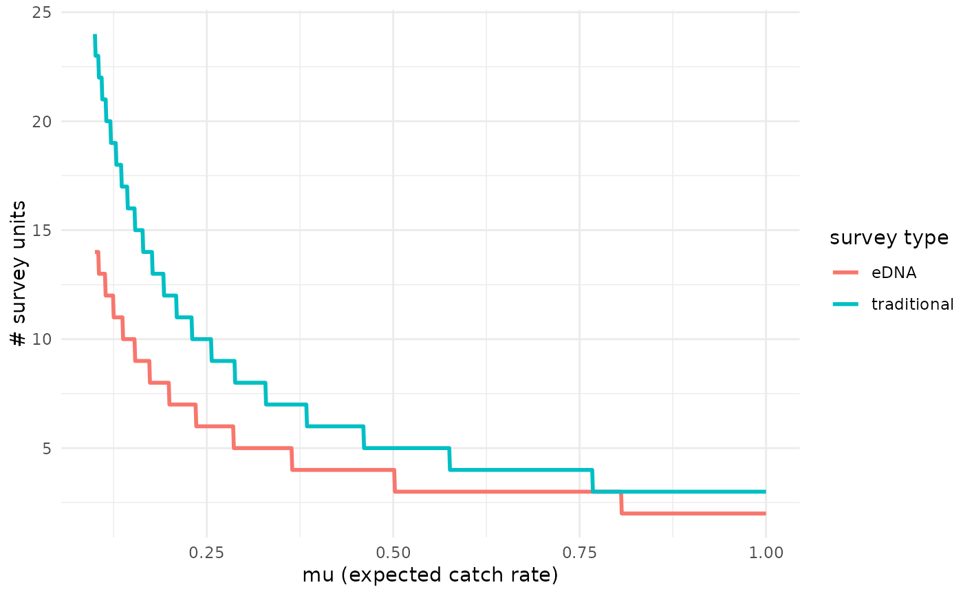
Plot the survey effort necessary to detect species presence, given the species expected catch rate.
Source:R/detection_plot.R
detection_plot.RdThis function plots the number of survey effort units to necessary detect species presence, calculated using median estimated parameter values from joint_model(). Detecting species presence is defined as producing at least one true positive eDNA detection or catching at least one individual. See more examples in the Package Vignette.
Arguments
- model_fit
An object of class
stanfit.- mu_min
A value indicating the minimum expected species catch rate for plotting. If multiple traditional gear types are represented in the model, mu is the catch rate of gear type 1.
- mu_max
A value indicating the maximum expected species catch rate for plotting. If multiple traditional gear types are represented in the model, mu is the catch rate of gear type 1.
- cov_val
A numeric vector indicating the values of site-level covariates to use for prediction. Default is NULL.
- probability
A numeric value indicating the probability of detecting presence. The default is 0.9.
- pcr_n
An integer indicating the number of PCR replicates per eDNA sample. The default is 3.
Value
A plot displaying survey efforts necessary to detect species presence, given mu, for each survey type.
Note
Before fitting the model, this function checks to ensure that the function is possible given the inputs. These checks include:
Input model fit is an object of class 'stanfit'.
Input mu_min is a numeric value greater than 0.
Input mu_max is a numeric value.
If model fit contains alpha, cov_val must be provided.
Input cov_val is numeric.
Input cov_val is the same length as the number of estimated covariates.
Input probability is a univariate numeric value.
Input model fit has converged (i.e. no divergent transitions after warm-up).
If any of these checks fail, the function returns an error message.
Examples
# \donttest{
# Ex. 1: Calculating necessary effort for detection with site-level
# covariates
# Load data
data(goby_data)
# Fit a model including 'Filter_time' and 'Salinity' site-level covariates
fit_cov <- joint_model(data = goby_data, cov = c('Filter_time','Salinity'),
family = "poisson", p10_priors = c(1,20), q = FALSE,
multicore = FALSE)
#>
#> SAMPLING FOR MODEL 'joint_count' NOW (CHAIN 1).
#> Chain 1:
#> Chain 1: Gradient evaluation took 3.4e-05 seconds
#> Chain 1: 1000 transitions using 10 leapfrog steps per transition would take 0.34 seconds.
#> Chain 1: Adjust your expectations accordingly!
#> Chain 1:
#> Chain 1:
#> Chain 1: Iteration: 1 / 3000 [ 0%] (Warmup)
#> Chain 1: Iteration: 500 / 3000 [ 16%] (Warmup)
#> Chain 1: Iteration: 501 / 3000 [ 16%] (Sampling)
#> Chain 1: Iteration: 1000 / 3000 [ 33%] (Sampling)
#> Chain 1: Iteration: 1500 / 3000 [ 50%] (Sampling)
#> Chain 1: Iteration: 2000 / 3000 [ 66%] (Sampling)
#> Chain 1: Iteration: 2500 / 3000 [ 83%] (Sampling)
#> Chain 1: Iteration: 3000 / 3000 [100%] (Sampling)
#> Chain 1:
#> Chain 1: Elapsed Time: 0.432 seconds (Warm-up)
#> Chain 1: 0.896 seconds (Sampling)
#> Chain 1: 1.328 seconds (Total)
#> Chain 1:
#>
#> SAMPLING FOR MODEL 'joint_count' NOW (CHAIN 2).
#> Chain 2:
#> Chain 2: Gradient evaluation took 2.9e-05 seconds
#> Chain 2: 1000 transitions using 10 leapfrog steps per transition would take 0.29 seconds.
#> Chain 2: Adjust your expectations accordingly!
#> Chain 2:
#> Chain 2:
#> Chain 2: Iteration: 1 / 3000 [ 0%] (Warmup)
#> Chain 2: Iteration: 500 / 3000 [ 16%] (Warmup)
#> Chain 2: Iteration: 501 / 3000 [ 16%] (Sampling)
#> Chain 2: Iteration: 1000 / 3000 [ 33%] (Sampling)
#> Chain 2: Iteration: 1500 / 3000 [ 50%] (Sampling)
#> Chain 2: Iteration: 2000 / 3000 [ 66%] (Sampling)
#> Chain 2: Iteration: 2500 / 3000 [ 83%] (Sampling)
#> Chain 2: Iteration: 3000 / 3000 [100%] (Sampling)
#> Chain 2:
#> Chain 2: Elapsed Time: 0.421 seconds (Warm-up)
#> Chain 2: 0.896 seconds (Sampling)
#> Chain 2: 1.317 seconds (Total)
#> Chain 2:
#>
#> SAMPLING FOR MODEL 'joint_count' NOW (CHAIN 3).
#> Chain 3:
#> Chain 3: Gradient evaluation took 2.8e-05 seconds
#> Chain 3: 1000 transitions using 10 leapfrog steps per transition would take 0.28 seconds.
#> Chain 3: Adjust your expectations accordingly!
#> Chain 3:
#> Chain 3:
#> Chain 3: Iteration: 1 / 3000 [ 0%] (Warmup)
#> Chain 3: Iteration: 500 / 3000 [ 16%] (Warmup)
#> Chain 3: Iteration: 501 / 3000 [ 16%] (Sampling)
#> Chain 3: Iteration: 1000 / 3000 [ 33%] (Sampling)
#> Chain 3: Iteration: 1500 / 3000 [ 50%] (Sampling)
#> Chain 3: Iteration: 2000 / 3000 [ 66%] (Sampling)
#> Chain 3: Iteration: 2500 / 3000 [ 83%] (Sampling)
#> Chain 3: Iteration: 3000 / 3000 [100%] (Sampling)
#> Chain 3:
#> Chain 3: Elapsed Time: 0.656 seconds (Warm-up)
#> Chain 3: 46.264 seconds (Sampling)
#> Chain 3: 46.92 seconds (Total)
#> Chain 3:
#>
#> SAMPLING FOR MODEL 'joint_count' NOW (CHAIN 4).
#> Chain 4:
#> Chain 4: Gradient evaluation took 3.3e-05 seconds
#> Chain 4: 1000 transitions using 10 leapfrog steps per transition would take 0.33 seconds.
#> Chain 4: Adjust your expectations accordingly!
#> Chain 4:
#> Chain 4:
#> Chain 4: Iteration: 1 / 3000 [ 0%] (Warmup)
#> Chain 4: Iteration: 500 / 3000 [ 16%] (Warmup)
#> Chain 4: Iteration: 501 / 3000 [ 16%] (Sampling)
#> Chain 4: Iteration: 1000 / 3000 [ 33%] (Sampling)
#> Chain 4: Iteration: 1500 / 3000 [ 50%] (Sampling)
#> Chain 4: Iteration: 2000 / 3000 [ 66%] (Sampling)
#> Chain 4: Iteration: 2500 / 3000 [ 83%] (Sampling)
#> Chain 4: Iteration: 3000 / 3000 [100%] (Sampling)
#> Chain 4:
#> Chain 4: Elapsed Time: 0.407 seconds (Warm-up)
#> Chain 4: 0.899 seconds (Sampling)
#> Chain 4: 1.306 seconds (Total)
#> Chain 4:
#> Warning: There were 199 divergent transitions after warmup. See
#> https://mc-stan.org/misc/warnings.html#divergent-transitions-after-warmup
#> to find out why this is a problem and how to eliminate them.
#> Warning: There were 2301 transitions after warmup that exceeded the maximum treedepth. Increase max_treedepth above 10. See
#> https://mc-stan.org/misc/warnings.html#maximum-treedepth-exceeded
#> Warning: There were 1 chains where the estimated Bayesian Fraction of Missing Information was low. See
#> https://mc-stan.org/misc/warnings.html#bfmi-low
#> Warning: Examine the pairs() plot to diagnose sampling problems
#> Warning: The largest R-hat is 1.06, indicating chains have not mixed.
#> Running the chains for more iterations may help. See
#> https://mc-stan.org/misc/warnings.html#r-hat
#> Warning: Bulk Effective Samples Size (ESS) is too low, indicating posterior means and medians may be unreliable.
#> Running the chains for more iterations may help. See
#> https://mc-stan.org/misc/warnings.html#bulk-ess
#> Warning: Tail Effective Samples Size (ESS) is too low, indicating posterior variances and tail quantiles may be unreliable.
#> Running the chains for more iterations may help. See
#> https://mc-stan.org/misc/warnings.html#tail-ess
#> Refer to the eDNAjoint guide for visualization tips: https://ednajoint.netlify.app/tips#visualization-tips
# Plot at the mean covariate values (covariates are standardized, so mean=0)
detection_plot(fit_cov$model, mu_min = 0.1, mu_max = 1,
cov_val = c(0,0), pcr_n = 3)
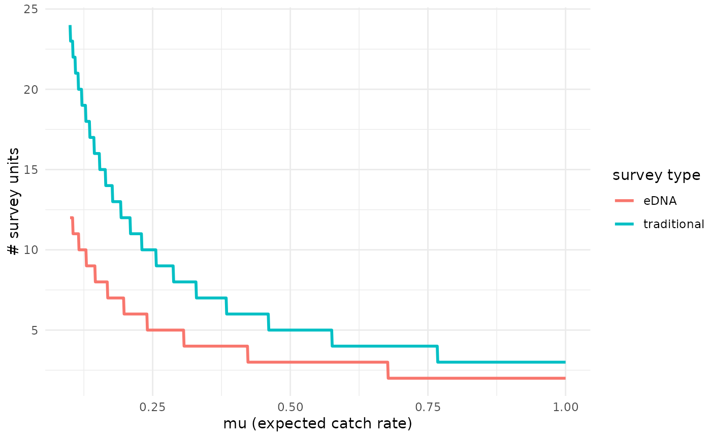
 # Calculate mu_critical at salinity 0.5 z-scores greater than the mean
detection_plot(fit_cov$model, mu_min = 0.1, mu_max = 1, cov_val = c(0,0.5),
pcr_n = 3)
# Calculate mu_critical at salinity 0.5 z-scores greater than the mean
detection_plot(fit_cov$model, mu_min = 0.1, mu_max = 1, cov_val = c(0,0.5),
pcr_n = 3)
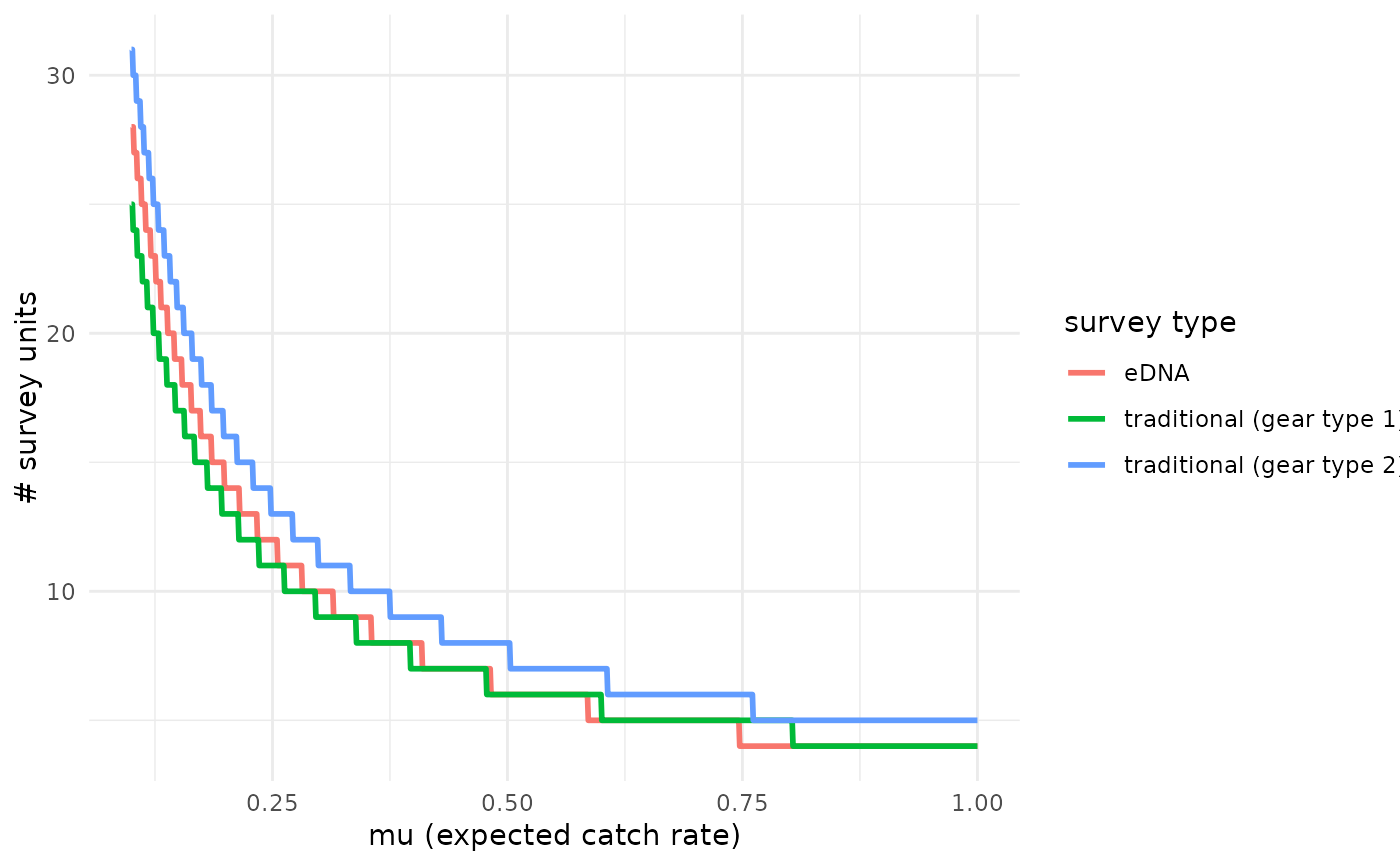
 # Ex. 2: Calculating necessary effort for detection with multiple
# traditional gear types
# Load data
data(green_crab_data)
# Fit a model with no site-level covariates
fit_q <- joint_model(data = green_crab_data, cov = NULL, family = "negbin",
p10_priors = c(1,20), q = TRUE,
multicore = FALSE)
#>
#> SAMPLING FOR MODEL 'joint_count' NOW (CHAIN 1).
#> Chain 1:
#> Chain 1: Gradient evaluation took 0.000444 seconds
#> Chain 1: 1000 transitions using 10 leapfrog steps per transition would take 4.44 seconds.
#> Chain 1: Adjust your expectations accordingly!
#> Chain 1:
#> Chain 1:
#> Chain 1: Iteration: 1 / 3000 [ 0%] (Warmup)
#> Chain 1: Iteration: 500 / 3000 [ 16%] (Warmup)
#> Chain 1: Iteration: 501 / 3000 [ 16%] (Sampling)
#> Chain 1: Iteration: 1000 / 3000 [ 33%] (Sampling)
#> Chain 1: Iteration: 1500 / 3000 [ 50%] (Sampling)
#> Chain 1: Iteration: 2000 / 3000 [ 66%] (Sampling)
#> Chain 1: Iteration: 2500 / 3000 [ 83%] (Sampling)
#> Chain 1: Iteration: 3000 / 3000 [100%] (Sampling)
#> Chain 1:
#> Chain 1: Elapsed Time: 4.969 seconds (Warm-up)
#> Chain 1: 16.302 seconds (Sampling)
#> Chain 1: 21.271 seconds (Total)
#> Chain 1:
#>
#> SAMPLING FOR MODEL 'joint_count' NOW (CHAIN 2).
#> Chain 2:
#> Chain 2: Gradient evaluation took 0.000406 seconds
#> Chain 2: 1000 transitions using 10 leapfrog steps per transition would take 4.06 seconds.
#> Chain 2: Adjust your expectations accordingly!
#> Chain 2:
#> Chain 2:
#> Chain 2: Iteration: 1 / 3000 [ 0%] (Warmup)
#> Chain 2: Iteration: 500 / 3000 [ 16%] (Warmup)
#> Chain 2: Iteration: 501 / 3000 [ 16%] (Sampling)
#> Chain 2: Iteration: 1000 / 3000 [ 33%] (Sampling)
#> Chain 2: Iteration: 1500 / 3000 [ 50%] (Sampling)
#> Chain 2: Iteration: 2000 / 3000 [ 66%] (Sampling)
#> Chain 2: Iteration: 2500 / 3000 [ 83%] (Sampling)
#> Chain 2: Iteration: 3000 / 3000 [100%] (Sampling)
#> Chain 2:
#> Chain 2: Elapsed Time: 4.828 seconds (Warm-up)
#> Chain 2: 14.549 seconds (Sampling)
#> Chain 2: 19.377 seconds (Total)
#> Chain 2:
#>
#> SAMPLING FOR MODEL 'joint_count' NOW (CHAIN 3).
#> Chain 3:
#> Chain 3: Gradient evaluation took 0.00044 seconds
#> Chain 3: 1000 transitions using 10 leapfrog steps per transition would take 4.4 seconds.
#> Chain 3: Adjust your expectations accordingly!
#> Chain 3:
#> Chain 3:
#> Chain 3: Iteration: 1 / 3000 [ 0%] (Warmup)
#> Chain 3: Iteration: 500 / 3000 [ 16%] (Warmup)
#> Chain 3: Iteration: 501 / 3000 [ 16%] (Sampling)
#> Chain 3: Iteration: 1000 / 3000 [ 33%] (Sampling)
#> Chain 3: Iteration: 1500 / 3000 [ 50%] (Sampling)
#> Chain 3: Iteration: 2000 / 3000 [ 66%] (Sampling)
#> Chain 3: Iteration: 2500 / 3000 [ 83%] (Sampling)
#> Chain 3: Iteration: 3000 / 3000 [100%] (Sampling)
#> Chain 3:
#> Chain 3: Elapsed Time: 4.85 seconds (Warm-up)
#> Chain 3: 11.104 seconds (Sampling)
#> Chain 3: 15.954 seconds (Total)
#> Chain 3:
#>
#> SAMPLING FOR MODEL 'joint_count' NOW (CHAIN 4).
#> Chain 4:
#> Chain 4: Gradient evaluation took 0.000428 seconds
#> Chain 4: 1000 transitions using 10 leapfrog steps per transition would take 4.28 seconds.
#> Chain 4: Adjust your expectations accordingly!
#> Chain 4:
#> Chain 4:
#> Chain 4: Iteration: 1 / 3000 [ 0%] (Warmup)
#> Chain 4: Iteration: 500 / 3000 [ 16%] (Warmup)
#> Chain 4: Iteration: 501 / 3000 [ 16%] (Sampling)
#> Chain 4: Iteration: 1000 / 3000 [ 33%] (Sampling)
#> Chain 4: Iteration: 1500 / 3000 [ 50%] (Sampling)
#> Chain 4: Iteration: 2000 / 3000 [ 66%] (Sampling)
#> Chain 4: Iteration: 2500 / 3000 [ 83%] (Sampling)
#> Chain 4: Iteration: 3000 / 3000 [100%] (Sampling)
#> Chain 4:
#> Chain 4: Elapsed Time: 4.723 seconds (Warm-up)
#> Chain 4: 11.681 seconds (Sampling)
#> Chain 4: 16.404 seconds (Total)
#> Chain 4:
#> Refer to the eDNAjoint guide for visualization tips: https://ednajoint.netlify.app/tips#visualization-tips
# Calculate
detection_plot(fit_q$model, mu_min = 0.1, mu_max = 1,
cov_val = NULL, pcr_n = 3)
# Ex. 2: Calculating necessary effort for detection with multiple
# traditional gear types
# Load data
data(green_crab_data)
# Fit a model with no site-level covariates
fit_q <- joint_model(data = green_crab_data, cov = NULL, family = "negbin",
p10_priors = c(1,20), q = TRUE,
multicore = FALSE)
#>
#> SAMPLING FOR MODEL 'joint_count' NOW (CHAIN 1).
#> Chain 1:
#> Chain 1: Gradient evaluation took 0.000444 seconds
#> Chain 1: 1000 transitions using 10 leapfrog steps per transition would take 4.44 seconds.
#> Chain 1: Adjust your expectations accordingly!
#> Chain 1:
#> Chain 1:
#> Chain 1: Iteration: 1 / 3000 [ 0%] (Warmup)
#> Chain 1: Iteration: 500 / 3000 [ 16%] (Warmup)
#> Chain 1: Iteration: 501 / 3000 [ 16%] (Sampling)
#> Chain 1: Iteration: 1000 / 3000 [ 33%] (Sampling)
#> Chain 1: Iteration: 1500 / 3000 [ 50%] (Sampling)
#> Chain 1: Iteration: 2000 / 3000 [ 66%] (Sampling)
#> Chain 1: Iteration: 2500 / 3000 [ 83%] (Sampling)
#> Chain 1: Iteration: 3000 / 3000 [100%] (Sampling)
#> Chain 1:
#> Chain 1: Elapsed Time: 4.969 seconds (Warm-up)
#> Chain 1: 16.302 seconds (Sampling)
#> Chain 1: 21.271 seconds (Total)
#> Chain 1:
#>
#> SAMPLING FOR MODEL 'joint_count' NOW (CHAIN 2).
#> Chain 2:
#> Chain 2: Gradient evaluation took 0.000406 seconds
#> Chain 2: 1000 transitions using 10 leapfrog steps per transition would take 4.06 seconds.
#> Chain 2: Adjust your expectations accordingly!
#> Chain 2:
#> Chain 2:
#> Chain 2: Iteration: 1 / 3000 [ 0%] (Warmup)
#> Chain 2: Iteration: 500 / 3000 [ 16%] (Warmup)
#> Chain 2: Iteration: 501 / 3000 [ 16%] (Sampling)
#> Chain 2: Iteration: 1000 / 3000 [ 33%] (Sampling)
#> Chain 2: Iteration: 1500 / 3000 [ 50%] (Sampling)
#> Chain 2: Iteration: 2000 / 3000 [ 66%] (Sampling)
#> Chain 2: Iteration: 2500 / 3000 [ 83%] (Sampling)
#> Chain 2: Iteration: 3000 / 3000 [100%] (Sampling)
#> Chain 2:
#> Chain 2: Elapsed Time: 4.828 seconds (Warm-up)
#> Chain 2: 14.549 seconds (Sampling)
#> Chain 2: 19.377 seconds (Total)
#> Chain 2:
#>
#> SAMPLING FOR MODEL 'joint_count' NOW (CHAIN 3).
#> Chain 3:
#> Chain 3: Gradient evaluation took 0.00044 seconds
#> Chain 3: 1000 transitions using 10 leapfrog steps per transition would take 4.4 seconds.
#> Chain 3: Adjust your expectations accordingly!
#> Chain 3:
#> Chain 3:
#> Chain 3: Iteration: 1 / 3000 [ 0%] (Warmup)
#> Chain 3: Iteration: 500 / 3000 [ 16%] (Warmup)
#> Chain 3: Iteration: 501 / 3000 [ 16%] (Sampling)
#> Chain 3: Iteration: 1000 / 3000 [ 33%] (Sampling)
#> Chain 3: Iteration: 1500 / 3000 [ 50%] (Sampling)
#> Chain 3: Iteration: 2000 / 3000 [ 66%] (Sampling)
#> Chain 3: Iteration: 2500 / 3000 [ 83%] (Sampling)
#> Chain 3: Iteration: 3000 / 3000 [100%] (Sampling)
#> Chain 3:
#> Chain 3: Elapsed Time: 4.85 seconds (Warm-up)
#> Chain 3: 11.104 seconds (Sampling)
#> Chain 3: 15.954 seconds (Total)
#> Chain 3:
#>
#> SAMPLING FOR MODEL 'joint_count' NOW (CHAIN 4).
#> Chain 4:
#> Chain 4: Gradient evaluation took 0.000428 seconds
#> Chain 4: 1000 transitions using 10 leapfrog steps per transition would take 4.28 seconds.
#> Chain 4: Adjust your expectations accordingly!
#> Chain 4:
#> Chain 4:
#> Chain 4: Iteration: 1 / 3000 [ 0%] (Warmup)
#> Chain 4: Iteration: 500 / 3000 [ 16%] (Warmup)
#> Chain 4: Iteration: 501 / 3000 [ 16%] (Sampling)
#> Chain 4: Iteration: 1000 / 3000 [ 33%] (Sampling)
#> Chain 4: Iteration: 1500 / 3000 [ 50%] (Sampling)
#> Chain 4: Iteration: 2000 / 3000 [ 66%] (Sampling)
#> Chain 4: Iteration: 2500 / 3000 [ 83%] (Sampling)
#> Chain 4: Iteration: 3000 / 3000 [100%] (Sampling)
#> Chain 4:
#> Chain 4: Elapsed Time: 4.723 seconds (Warm-up)
#> Chain 4: 11.681 seconds (Sampling)
#> Chain 4: 16.404 seconds (Total)
#> Chain 4:
#> Refer to the eDNAjoint guide for visualization tips: https://ednajoint.netlify.app/tips#visualization-tips
# Calculate
detection_plot(fit_q$model, mu_min = 0.1, mu_max = 1,
cov_val = NULL, pcr_n = 3)
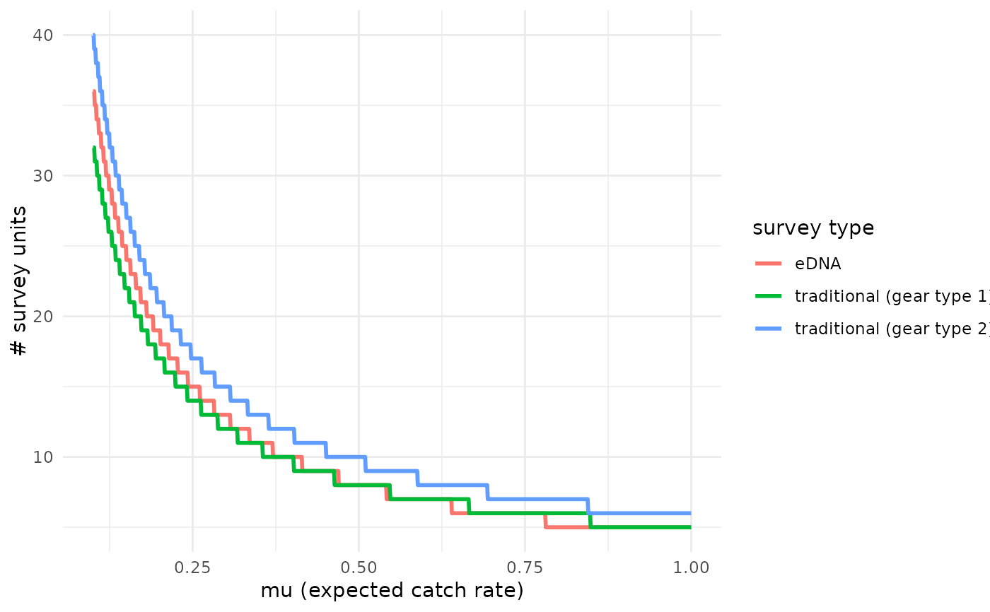
 # Change probability of detecting presence to 0.95
detection_plot(fit_q$model, mu_min = 0.1, mu_max = 1, cov_val = NULL,
probability = 0.95, pcr_n = 3)
# Change probability of detecting presence to 0.95
detection_plot(fit_q$model, mu_min = 0.1, mu_max = 1, cov_val = NULL,
probability = 0.95, pcr_n = 3)
 # }
# }