Plotting healthy life expectancy and life expectancy by deprivation for English local authorities
Source:vignettes/lifeExpectancy.Rmd
lifeExpectancy.Rmd
knitr::opts_chunk$set(fig.path = "charts-")This worked example attempts to document a common workflow a user
might follow when using the fingertipsR package.
fingertipsR provides users the ability to import data
from the Fingertips website.
Fingertips is a major repository of public health indicators in England.
The site is structured in the following way:
- Profiles - these contain indicators related to a broad theme (such as a risk factor or a disease topic etc)
- Domains - these are subcategories of profiles, and break the profiles down to themes within the broader theme
- Indicators - this is the lowest level of the structure and sit within the domains. Indicators are presented at different time periods, geographies, sexes, ageband and categories.
This example demonstrates how you can plot healthy life expectancy and life expectancy by geographical regions for a given year of data that fingertips contains. So, where to start?
Where to start
There is one function in the fingertipsR package that
imports data from the Fingertips API; fingertips_data().
This function has the following inputs:
- IndicatorID
- AreaCode
- DomainID
- ProfileID
- AreaTypeID
- ParentAreaTypeID
At least one of IndicatorID, DomainID or
ProfileID must be complete. These fields relate to each other
as described in the introduction. AreaTypeID is also required,
and determines the geography for which data is imported. In this case we
want County and Unitary Authority level. AreaCode needs
completing if you are extracting data for a particular area or group of
areas only. ParentAreaTypeID requires an area type code that
the AreaTypeID maps to at a higher level of geography. For
example, County and Unitary Authorities map to a higher level of
geography called Government Office Regions. These mappings can be
identified using the area_types() function. If ignored, a
ParentAreaTypeID will be chosen automatically.
Therefore, the inputs to the fingertips_data function
that we need to find out are the ID codes for:
- IndicatorID
- AreaTypeID
- ParentAreaTypeID
We need to begin by calling the fingertipsR package:
IndicatorID
There are two indicators we are interested in for this exercise. Without consulting the Fingertips website, we know approximately what they are called:
- Healthy life expectancy
- Life expectancy
We can use the indicators() function to return a list of
all the indicators within Fingertips. We can then filter the name field
for the term life expectancy (note, the IndicatorName field has
been converted to lower case in the following code chunk to ensure
matches will not be overlooked as a result of upper case letters).
inds <- indicators_unique()
life_expectancy <- inds[grepl("life expectancy", tolower(inds$IndicatorName)),]| IndicatorID | IndicatorName |
|---|---|
| 90362 | Healthy life expectancy at birth |
| 90366 | Life expectancy at birth |
| 90825 | Inequality in healthy life expectancy at birth ENGLAND |
| 91102 | Life expectancy at 65 |
| 92031 | Inequality in healthy life expectancy at birth LA |
| 92901 | Inequality in life expectancy at birth |
| 93190 | Inequality in life expectancy at 65 |
| 93505 | Healthy life expectancy at 65 |
| 93523 | Disability-free life expectancy at 65 |
| 93562 | Disability-free life expectancy at birth |
| 650 | Life expectancy - MSOA based |
| 93249 | Disability free life expectancy, (Upper age band 85+) |
| 93283 | Life expectancy at birth, (upper age band 90+) |
| 93285 | Life expectancy at birth, (upper age band 85+) |
| 93298 | Healthy life expectancy, (upper age band 85+) |
| 92641 | Life expectancy at 75 (SPOT: NHSOD 1b) |
| 90365 | Gap in life expectancy at birth between each local authority and England as a whole |
The two indicators we are interested in from this table are:
- 90362
- 90366
AreaTypeID
We can work out what the AreaTypeID codes we need using the
function area_types(). We’ve decided that we want to
produce the graph at County and Unitary Authority level. From the
section Where to start we need codes for
AreaTypeID and ParentAreaTypeID.
areaTypes <- area_types()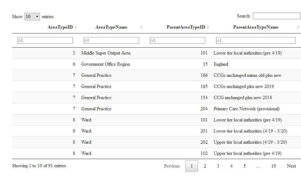
The table shows that the AreaTypeID for County and Unitary Authority level is 202. The third column, ParentAreaTypeID, shows the IDs of the area types that these map to. In the case of County and Unitary Authorities, these are:
| AreaTypeID | AreaTypeName | ParentAreaTypeID | ParentAreaTypeName |
|---|---|---|---|
| 202 | Counties & UAs (2019/20) | 6 | Government Office Region |
| 202 | Counties & UAs (2019/20) | 104 | PHEC 2015 new plus PHEC 2013 unchanged |
| 202 | Counties & UAs (2019/20) | 10105 | Depriv. decile (IMD2015, 4/19 boundaries) |
| 202 | Counties & UAs (2019/20) | 10113 | Depriv. deciles (IMD2019) |
| 202 | Counties & UAs (2019/20) | 126 | Combined authorities |
ParentAreaTypeID is 6 by default for the
fingertips_data() function for AreaTypeID of
202 (this value changes if different AreaTypeIDs are
entered), so we can stick with that in this example. Use the
area_types() function to understand more about how areas
map to each other.
Extracting the data
Finally, we can use the fingertips_data() function with
the inputs we have determined previously.
indicators <- c(90362, 90366)
data <- fingertips_data(IndicatorID = indicators,
                        AreaTypeID = 202)
##
##
## | | IndicatorID | IndicatorName | ParentCode |
## |:--------:|:-----------:|:------------------------:|:----------:|
## | **8023** | 90366 | Life expectancy at birth | E12000005 |
## | **8024** | 90366 | Life expectancy at birth | E12000006 |
## | **8025** | 90366 | Life expectancy at birth | E12000008 |
## | **8026** | 90366 | Life expectancy at birth | E12000005 |
## | **8027** | 90366 | Life expectancy at birth | E12000008 |
## | **8028** | 90366 | Life expectancy at birth | E12000005 |
##
## Table: Table continues below
##
##
##
## | | ParentName | AreaCode | AreaName |
## |:--------:|:----------------------:|:---------:|:--------------:|
## | **8023** | West Midlands region | E10000028 | Staffordshire |
## | **8024** | East of England region | E10000029 | Suffolk |
## | **8025** | South East region | E10000030 | Surrey |
## | **8026** | West Midlands region | E10000031 | Warwickshire |
## | **8027** | South East region | E10000032 | West Sussex |
## | **8028** | West Midlands region | E10000034 | Worcestershire |
##
## Table: Table continues below
##
##
##
## | | AreaType | Sex | Age | CategoryType | Category |
## |:--------:|:-----------------------:|:------:|:--------:|:------------:|:--------:|
## | **8023** | County & UA (4/19-3/20) | Female | All ages | NA | NA |
## | **8024** | County & UA (4/19-3/20) | Female | All ages | NA | NA |
## | **8025** | County & UA (4/19-3/20) | Female | All ages | NA | NA |
## | **8026** | County & UA (4/19-3/20) | Female | All ages | NA | NA |
## | **8027** | County & UA (4/19-3/20) | Female | All ages | NA | NA |
## | **8028** | County & UA (4/19-3/20) | Female | All ages | NA | NA |
##
## Table: Table continues below
##
##
##
## | | Timeperiod | Value | LowerCI95.0limit | UpperCI95.0limit |
## |:--------:|:----------:|:-----:|:----------------:|:----------------:|
## | **8023** | 2017 - 19 | 83.45 | 83.24 | 83.66 |
## | **8024** | 2017 - 19 | 84.25 | 84.02 | 84.47 |
## | **8025** | 2017 - 19 | 85.33 | 85.15 | 85.51 |
## | **8026** | 2017 - 19 | 83.85 | 83.58 | 84.11 |
## | **8027** | 2017 - 19 | 84.21 | 84 | 84.42 |
## | **8028** | 2017 - 19 | 83.8 | 83.54 | 84.06 |
##
## Table: Table continues below
##
##
##
## | | LowerCI99.8limit | UpperCI99.8limit | Count | Denominator | Valuenote |
## |:--------:|:----------------:|:----------------:|:-----:|:-----------:|:---------:|
## | **8023** | NA | NA | NA | NA | NA |
## | **8024** | NA | NA | NA | NA | NA |
## | **8025** | NA | NA | NA | NA | NA |
## | **8026** | NA | NA | NA | NA | NA |
## | **8027** | NA | NA | NA | NA | NA |
## | **8028** | NA | NA | NA | NA | NA |
##
## Table: Table continues below
##
##
##
## | | RecentTrend | ComparedtoEnglandvalueorpercentiles |
## |:--------:|:--------------------:|:-----------------------------------:|
## | **8023** | Cannot be calculated | Similar |
## | **8024** | Cannot be calculated | Better |
## | **8025** | Cannot be calculated | Better |
## | **8026** | Cannot be calculated | Better |
## | **8027** | Cannot be calculated | Better |
## | **8028** | Cannot be calculated | Better |
##
## Table: Table continues below
##
##
##
## | | ComparedtoRegionvalueorpercentiles | TimeperiodSortable | Newdata |
## |:--------:|:----------------------------------:|:------------------:|:-------:|
## | **8023** | Better | 20170000 | NA |
## | **8024** | Better | 20170000 | NA |
## | **8025** | Better | 20170000 | NA |
## | **8026** | Better | 20170000 | NA |
## | **8027** | Similar | 20170000 | NA |
## | **8028** | Better | 20170000 | NA |
##
## Table: Table continues below
##
##
##
## | | Comparedtogoal |
## |:--------:|:--------------:|
## | **8023** | NA |
## | **8024** | NA |
## | **8025** | NA |
## | **8026** | NA |
## | **8027** | NA |
## | **8028** | NA |The data frame returned by fingertips_data() contains 26
variables. For this exercise, we are only interested in a few of them
and for the time period 2012-14:
- IndicatorID
- AreaCode
- ParentAreaName
- Sex
- Timeperiod
- Value
The data frame also contains data for the parent area, and for England, so we want to filter it to remove these too.
cols <- c("IndicatorID", "AreaCode", "ParentName", "Sex", "Timeperiod", "Value")

area_type_name <- table(data$AreaType) # tally each group in the AreaType field

area_type_name <- area_type_name[area_type_name == max(area_type_name)] # pick the group with the highest frequency
area_type_name <- names(area_type_name) # retrieve the name

data <- data[data$AreaType == area_type_name &
               data$Timeperiod == "2012 - 14", cols]
Plotting outputs
Using ggplot2 it is possible to plot the outputs.
library(ggplot2)
ggplot(data, aes(x = reorder(ParentName, Value, median), y = Value, col = factor(IndicatorID))) +
        geom_boxplot(data = data[data$IndicatorID == 90366, ]) +
        geom_boxplot(data = data[data$IndicatorID == 90362, ]) +
        facet_wrap(~ Sex) +
        scale_colour_manual(name = "Indicator",
                            breaks = c("90366", "90362"),
                            labels = c("Life expectancy", "Healthy life expectancy"),
                            values = c("#128c4a", "#88c857")) +
        labs(x = "Region",
             y = "Age",
             title = "Life expectancy and healthy life expectancy at birth \nfor Upper Tier Local Authorities within England regions (2012 - 2014)") +
        theme_bw() +
        theme(axis.text.x = element_text(angle = 45,
                                         hjust = 1))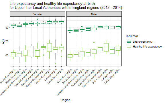
Other useful functions
The plot above makes use of the fields that are within the dataset by
default when using the fingertips_data() function. There is
also a deprivation_decile() function, which provides an
indicator of deprivation for each geographical area (see
?deprivation_decile).
Not all indicators are available for every geography. To understand
how indicators are mapped to different gegoraphies, there is a function
indicator_areatypes().
To understand more about what comprises each indicator, there is the
indicator_metadata() function, which provides the
information on the definitions page of the Fingertips website.
Finally, the nearest_neighbours() function provides
groups of statistically similar area for some of the geographies that
are available. The geographies these are available for, and their
sources, are documented within the function documentation
(?nearest_neighbours).