The R package forcis is an interface to the FORCIS database
on global foraminifera distribution (Chaabane et al. 2023). This
database includes data on living planktonic foraminifera diversity and
distribution in the global oceans from 1910 until 2018 collected using
plankton tows, continuous plankton recorder, sediment traps and plankton
pump from the global ocean.
This package has been developed for researchers interested in working with the FORCIS database, even without advanced R skills. It provides basic functions to facilitate the handling of this large database, including functions to download, select, filter, homogenize, and visualize the data. It also enables users to explore the spatial distribution and temporal evolution of planktonic foraminifera.
This vignette is an overview of the main features of the package.
Installation
To install the forcis package, run:
## Install < remotes > package (if not already installed) ----
if (!requireNamespace("remotes", quietly = TRUE)) {
  install.packages("remotes")
}

## Install dev version of < forcis > from GitHub ----
remotes::install_github("FRBCesab/forcis")
The
forcispackage depends on thesfpackage which requires some spatial system libraries (GDAL and PROJ). Please read this page if you have any trouble to installforcis.
Now let’s attach the required packages.
Download FORCIS database
The FORCIS database consists of a collection of five csv
files hosted on Zenodo. These
csv are regularly updated and we recommend to use the
latest version
Let’s download the latest version of the FORCIS database with
download_forcis_db():
# Create a data/ folder in the current directory ----
dir.create("data")

# Download latest version of the database ----
download_forcis_db(
  path = "data",
  version = NULL
)
By default (i.e. version = NULL), this function
downloads the latest version of the database. The database is saved in
data/forcis-db/version-99/, where 99 is the
version number.
N.B. The package forcis is designed to
handle the versioning of the database on Zenodo. Read the Database
versions for more information.
Import FORCIS data
In this vignette, we will use the plankton nets data of the FORCIS database. Let’s import the latest release of the data.
# Import plankton nets data ----
net_data <- read_plankton_nets_data(path = "data")
# Print data ----
net_data
#> # A tibble: 2,451 × 86
#>    data_type cruise_id    profile_id sample_id sample_min_depth sample_max_depth
#>    <chr>     <chr>        <chr>      <chr>                <dbl>            <dbl>
#>  1 Net       ATLANTIS_II… ATLANTIS_… ATLANTIS…                0               86
#>  2 Net       ATLANTIS_II… ATLANTIS_… ATLANTIS…                0               86
#>  3 Net       ATLANTIS_II… ATLANTIS_… ATLANTIS…                0              118
#>  4 Net       ATLANTIS_II… ATLANTIS_… ATLANTIS…                0              106
#>  5 Net       ATLANTIS_II… ATLANTIS_… ATLANTIS…                0              118
#>  6 Net       ATLANTIS_II… ATLANTIS_… ATLANTIS…                0               86
#>  7 Net       ATLANTIS_II… ATLANTIS_… ATLANTIS…                0               64
#>  8 Net       ATLANTIS_II… ATLANTIS_… ATLANTIS…                0               73
#>  9 Net       ATLANTIS_II… ATLANTIS_… ATLANTIS…                0               83
#> 10 Net       ATLANTIS_II… ATLANTIS_… ATLANTIS…                0              127
#> # ℹ 2,441 more rows
#> # ℹ 80 more variables: profile_depth_min <int>, profile_depth_max <dbl>,
#> #   profile_date_time <chr>, cast_net_op_m2 <dbl>, subsample_id <chr>,
#> #   sample_segment_length <lgl>, subsample_count_type <chr>,
#> #   subsample_size_fraction_min <int>, subsample_size_fraction_max <int>,
#> #   site_lat_start_decimal <dbl>, site_lon_start_decimal <dbl>,
#> #   sample_volume_filtered <dbl>, …
N.B. For this vignette, we use a subset of the plankton nets data, not the whole dataset.
Select a FORCIS taxonomy
The FORCIS database provides three different taxonomies:
-
OT: original taxonomy, i.e. the initial list of species names and attributes (e.g., shell pigmentation, coiling direction) as reported in various datasets and studies. -
VT: validated taxonomy, i.e. a refined version of the original taxonomy that resolves issues of synonymy (different names for the same taxon) and shifting taxonomic concepts. -
LT: lumped taxonomy, i.e. a simplified version of the validated taxonomy. It merges taxa that are difficult to distinguish across datasets (morphospecies), ensuring consistency and comparability in broader analyses.
See the associated data paper for further information.
After importing the data and before going any further, the next step involves choosing the taxonomic level for the analyses. This is mandatory to avoid duplicated records.
Let’s use the function select_taxonomy() to select the
VT taxonomy (validated taxonomy):
# Select taxonomy ----
net_data_vt <- net_data |>
  select_taxonomy(taxonomy = "VT")

net_data_vt
#> # A tibble: 2,451 × 80
#>    data_type cruise_id    profile_id sample_id sample_min_depth sample_max_depth
#>    <chr>     <chr>        <chr>      <chr>                <dbl>            <dbl>
#>  1 Net       ATLANTIS_II… ATLANTIS_… ATLANTIS…                0               86
#>  2 Net       ATLANTIS_II… ATLANTIS_… ATLANTIS…                0               86
#>  3 Net       ATLANTIS_II… ATLANTIS_… ATLANTIS…                0              118
#>  4 Net       ATLANTIS_II… ATLANTIS_… ATLANTIS…                0              106
#>  5 Net       ATLANTIS_II… ATLANTIS_… ATLANTIS…                0              118
#>  6 Net       ATLANTIS_II… ATLANTIS_… ATLANTIS…                0               86
#>  7 Net       ATLANTIS_II… ATLANTIS_… ATLANTIS…                0               64
#>  8 Net       ATLANTIS_II… ATLANTIS_… ATLANTIS…                0               73
#>  9 Net       ATLANTIS_II… ATLANTIS_… ATLANTIS…                0               83
#> 10 Net       ATLANTIS_II… ATLANTIS_… ATLANTIS…                0              127
#> # ℹ 2,441 more rows
#> # ℹ 74 more variables: profile_depth_min <int>, profile_depth_max <dbl>,
#> #   profile_date_time <chr>, cast_net_op_m2 <dbl>, subsample_id <chr>,
#> #   sample_segment_length <lgl>, subsample_count_type <chr>,
#> #   subsample_size_fraction_min <int>, subsample_size_fraction_max <int>,
#> #   site_lat_start_decimal <dbl>, site_lon_start_decimal <dbl>,
#> #   sample_volume_filtered <dbl>, …
This function has removed species columns associated with other taxonomies.
At this stage user can choose what he/she wants to do with this cleaned dataset. In the next sections, we present some use cases.
Use case 1: Exploration
In this first use case, we want to have an overview of our data.
# How many subsamples do we have? ----
nrow(net_data_vt)
#> [1] 2451

# How many species have been sampled? ----
net_data_vt |>
  get_species_names() |>
  length()
#> [1] 56
We can use the plot_record_by_year() function to display
the number of samples per year.
# What is the temporal extent? ----
plot_record_by_year(net_data_vt)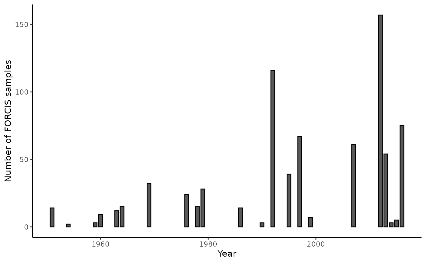
The plot_record_by_month() and
plot_record_by_season() are also available to display
samples at different temporal resolutions.
Let’s use the ggmap_data() function to get an idea of
the spatial extent of these data.
# What is the spatial extent? ----
ggmap_data(net_data_vt)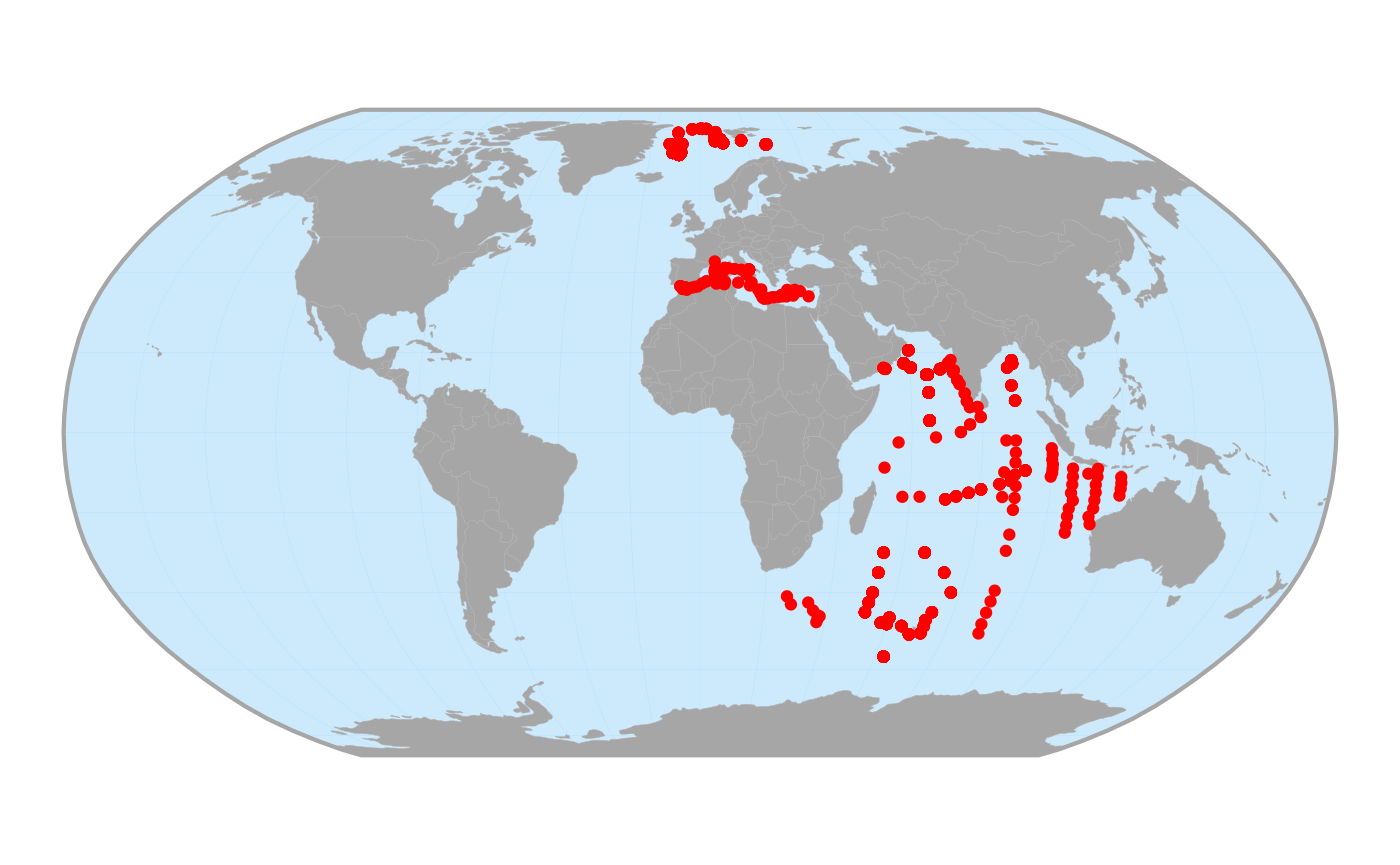
The Data
visualization vignette provides a complete description of all
plotting functions available in forcis.
Use case 2: Specific question
In this second use case we want to answer the following question:
What is the distribution of the planktonic foraminifera species Neogloboquadrina pachyderma between 1970 and 2000 in the Mediterranean Sea?
We can divide the problem into different stages:
- Find the species name in the FORCIS dataset
- Filter data for N. pachyderma
- Keep non-zero samples for this species
- Filter data for 1970-2000
- Filter data for Mediterranean Sea
- Plot records on a map
Find the species name
# Get all species names ----
species_list <- net_data_vt |>
  get_species_names()

# Search for species containing the word 'pachyderma' ----
species_list[grep("pachyderma", species_list)]
#> [1] "n_pachyderma_VT"          "n_pachyderma_incompta_VT"

# Store the species name ----
sp_name <- "n_pachyderma_VT"
Species filter
# Filter data by species ----
net_data_vt_pachyderma <- net_data_vt |>
  filter_by_species(species = sp_name)

net_data_vt_pachyderma
#> # A tibble: 2,451 × 25
#>    data_type cruise_id    profile_id sample_id sample_min_depth sample_max_depth
#>    <chr>     <chr>        <chr>      <chr>                <dbl>            <dbl>
#>  1 Net       ATLANTIS_II… ATLANTIS_… ATLANTIS…                0               86
#>  2 Net       ATLANTIS_II… ATLANTIS_… ATLANTIS…                0               86
#>  3 Net       ATLANTIS_II… ATLANTIS_… ATLANTIS…                0              118
#>  4 Net       ATLANTIS_II… ATLANTIS_… ATLANTIS…                0              106
#>  5 Net       ATLANTIS_II… ATLANTIS_… ATLANTIS…                0              118
#>  6 Net       ATLANTIS_II… ATLANTIS_… ATLANTIS…                0               86
#>  7 Net       ATLANTIS_II… ATLANTIS_… ATLANTIS…                0               64
#>  8 Net       ATLANTIS_II… ATLANTIS_… ATLANTIS…                0               73
#>  9 Net       ATLANTIS_II… ATLANTIS_… ATLANTIS…                0               83
#> 10 Net       ATLANTIS_II… ATLANTIS_… ATLANTIS…                0              127
#> # ℹ 2,441 more rows
#> # ℹ 19 more variables: profile_depth_min <int>, profile_depth_max <dbl>,
#> #   profile_date_time <chr>, cast_net_op_m2 <dbl>, subsample_id <chr>,
#> #   sample_segment_length <lgl>, subsample_count_type <chr>,
#> #   subsample_size_fraction_min <int>, subsample_size_fraction_max <int>,
#> #   site_lat_start_decimal <dbl>, site_lon_start_decimal <dbl>,
#> #   sample_volume_filtered <dbl>, …

# Remove empty samples for N. pachyderma ----
net_data_vt_pachyderma <- net_data_vt_pachyderma |>
  dplyr::filter(n_pachyderma_VT > 0)

net_data_vt_pachyderma
#> # A tibble: 823 × 25
#>    data_type cruise_id profile_id    sample_id sample_min_depth sample_max_depth
#>    <chr>     <chr>     <chr>         <chr>                <dbl>            <dbl>
#>  1 Net       NIOP-C1   NIOP-C1_309-… NIOP-C1_…             28.3             49.5
#>  2 Net       NIOP-C1   NIOP-C1_309-… NIOP-C1_…              8               18.2
#>  3 Net       NIOP-C1   NIOP-C1_310-… NIOP-C1_…             74.3             99.6
#>  4 Net       NIOP-C1   NIOP-C1_310-… NIOP-C1_…             48.5             74.3
#>  5 Net       NIOP-C1   NIOP-C1_310-… NIOP-C1_…             23.3             48.5
#>  6 Net       NIOP-C1   NIOP-C1_310-… NIOP-C1_…              8.1             23.3
#>  7 Net       NIOP-C1   NIOP-C1_310-… NIOP-C1_…            298.             498.
#>  8 Net       NIOP-C1   NIOP-C1_310-… NIOP-C1_…            200.             298.
#>  9 Net       NIOP-C1   NIOP-C1_310-… NIOP-C1_…            148.             200.
#> 10 Net       NIOP-C1   NIOP-C1_313-… NIOP-C1_…             74.8             99.6
#> # ℹ 813 more rows
#> # ℹ 19 more variables: profile_depth_min <int>, profile_depth_max <dbl>,
#> #   profile_date_time <chr>, cast_net_op_m2 <dbl>, subsample_id <chr>,
#> #   sample_segment_length <lgl>, subsample_count_type <chr>,
#> #   subsample_size_fraction_min <int>, subsample_size_fraction_max <int>,
#> #   site_lat_start_decimal <dbl>, site_lon_start_decimal <dbl>,
#> #   sample_volume_filtered <dbl>, …
Temporal filter
# Filter data by years ----
net_data_vt_pachyderma_7000 <- net_data_vt_pachyderma |>
  filter_by_year(years = 1970:2000)

# Number of records ----
nrow(net_data_vt_pachyderma_7000)
#> [1] 461
Spatial filter
# Get the list of ocean names ----
get_ocean_names()
#> [1] "Arctic Ocean"         "Indian Ocean"         "Mediterranean Sea"
#> [4] "North Atlantic Ocean" "North Pacific Ocean"  "South Atlantic Ocean"
#> [7] "South Pacific Ocean"  "Southern Ocean"

# Filter data by ocean ----
net_data_vt_pachyderma_7000_med <- net_data_vt_pachyderma_7000 |>
  filter_by_ocean(ocean = "Mediterranean Sea")

# Number of records ----
nrow(net_data_vt_pachyderma_7000_med)
#> [1] 2
Distribution map
# Plot N. pachyderma records on a World map ----
ggmap_data(net_data_vt_pachyderma_7000_med)
Finally, we can combine all these steps into one single pipeline:
# Final use case 2 code ----
net_data_vt |>
  filter_by_species(species = "n_pachyderma_VT") |>
  dplyr::filter(n_pachyderma_VT > 0) |>
  filter_by_year(years = 1970:2000) |>
  filter_by_ocean(ocean = "Mediterranean Sea") |>
  ggmap_data()
The Select, reshape, and filter data vignette shows examples to handle FORCIS data.
To go further
Additional vignettes are available depending on user wishes:
- the Database versions vignette provides information on how to deal with the versioning of the database
- the Select, reshape, and filter data vignette shows examples to select, filter and reshape the FORCIS data
- the Data
conversion vignette describes the conversion functions available in
forcisto compute abundances, concentrations, and frequencies - the Data
visualization vignette describes the plotting functions available in
forcis
References
Chaabane S, De Garidel-Thoron T, Giraud X, Schiebel R, Beaugrand G, Brummer G-J, Casajus N, Greco M, Grigoratou M, Howa H, Jonkers L, Kucera M, Kuroyanagi A, Meilland J, Monteiro F, Mortyn G, Almogi-Labin A, Asahi H, Avnaim-Katav S, Bassinot F, Davis CV, Field DB, Hernández-Almeida I, Herut B, Hosie G, Howard W, Jentzen A, Johns DG, Keigwin L, Kitchener J, Kohfeld KE, Lessa DVO, Manno C, Marchant M, Ofstad S, Ortiz JD, Post A, Rigual-Hernandez A, Rillo MC, Robinson K, Sagawa T, Sierro F, Takahashi KT, Torfstein A, Venancio I, Yamasaki M & Ziveri P (2023) The FORCIS database: A global census of planktonic Foraminifera from ocean waters. Scientific Data, 10, 354. DOI: 10.1038/s41597-023-02264-2.