Transition towards Open Access

Following the template in OpenAlex’s oa-percentage tutorial, this vignette uses openalexR to answer:

How many of recent journal articles from the University of Pennsylvania are open access? And how many aren’t?

library(openalexR)
library(dplyr)
library(tidyr)
library(ggplot2)

We first need to find the openalex.id for University of Pennsylvania. We can do this by fetching for the institutions entity and put “University of Pennsylvania” in display_name or display_name.search:

oa_fetch(
  entity = "inst", # same as "institutions"
  display_name.search = "\"University of Pennsylvania\""
) %>%
  select(display_name, ror) %>% 
  knitr::kable()

display_name	ror
University of Pennsylvania	https://ror.org/00b30xv10
California University of Pennsylvania	https://ror.org/01spssf70
Hospital of the University of Pennsylvania	https://ror.org/02917wp91
University of Pennsylvania Health System	https://ror.org/04h81rw26
Indiana University of Pennsylvania	https://ror.org/0511cmw96
University of Pennsylvania Press	https://ror.org/03xwa9562
Cheyney University of Pennsylvania	https://ror.org/02nckwn80

We will use the first ror, 00b30xv10, as one of the filters for our query.

Alternatively, we could go to the autocomplete endpoint at https://explore.openalex.org/ to search for “University of Pennsylvania” and find the ror there!

All other filters are straightforward and explained in detailed in the original jupyter notebook tutorial. The only difference here is that, instead of grouping by is_oa, we’re interested in the “trend” over the years, so we’re going to group by publication_year, and perform the query twice, one for is_oa = "true" and one for is_oa = "false" .

open_access <- oa_fetch(
  entity = "works",
  institutions.ror = "00b30xv10",
  type = "article",
  from_publication_date = "2012-08-24",
  is_paratext = "false",
  is_oa = "true",
  group_by = "publication_year"
)

closed_access <- oa_fetch(
  entity = "works",
  institutions.ror = "00b30xv10",
  type = "article",
  from_publication_date = "2012-08-24",
  is_paratext = "false",
  is_oa = "false",
  group_by = "publication_year"
)

uf_df <- closed_access %>%
  select(- key_display_name) %>%
  full_join(open_access, by = "key", suffix = c("_ca", "_oa")) 

uf_df
#>     key count_ca key_display_name count_oa
#> 1  2018     4300             2018     5447
#> 2  2025     4131             2025     6956
#> 3  2022     4127             2022     7327
#> 4  2019     4091             2019     6220
#> 5  2020     4081             2020     7705
#> 6  2021     4030             2021     7842
#> 7  2024     3873             2024     7705
#> 8  2015     3829             2015     4528
#> 9  2014     3779             2014     4405
#> 10 2013     3677             2013     4380
#> 11 2016     3636             2016     4845
#> 12 2017     3592             2017     5177
#> 13 2023     3489             2023     8189
#> 14 2012     1156             2012     1148
#> 15 2026      305             2026      487

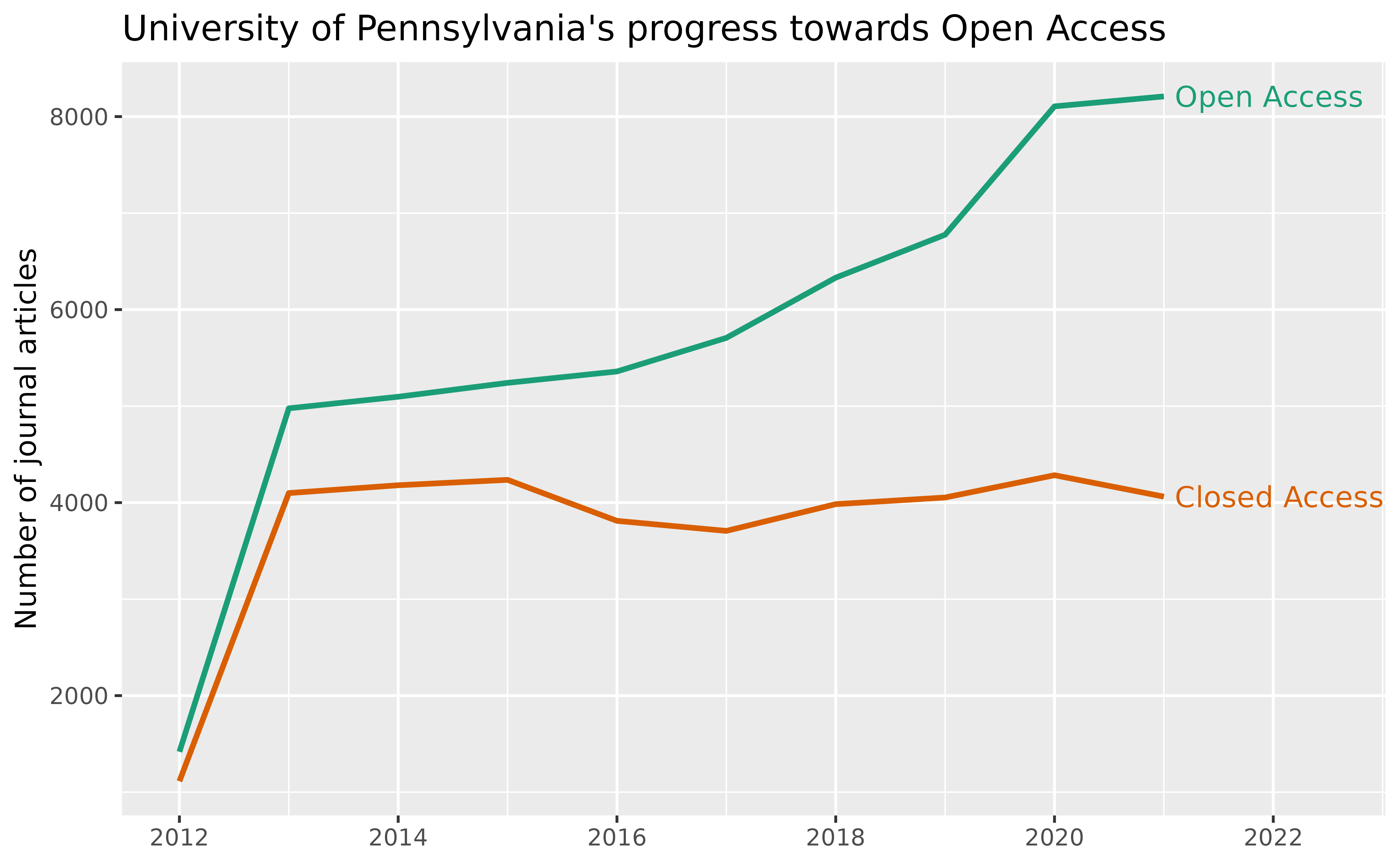
Finally, we compare the number of open vs. closed access articles over the years:

uf_df %>%
  filter(key <= 2021) %>% # we do not yet have complete data for 2022 and after
  pivot_longer(cols = starts_with("count")) %>%
  mutate(
    year = as.integer(key),
    is_oa = recode(
      name,
      "count_ca" = "Closed Access",
      "count_oa" = "Open Access"
    ),
    label = if_else(key < 2021, NA_character_, is_oa)
  ) %>% 
  select(year, value, is_oa, label) %>%
  ggplot(aes(x = year, y = value, group = is_oa, color = is_oa)) +
  geom_line(size = 1) +
  labs(
    title = "University of Pennsylvania's progress towards Open Access",
    x = NULL, y = "Number of journal articles") +
  scale_color_brewer(palette = "Dark2", direction = -1) +
  scale_x_continuous(breaks = seq(2010, 2024, 2)) +
  geom_text(aes(label = label), nudge_x = 0.1, hjust = 0) +
  coord_cartesian(xlim = c(NA, 2022.5)) +
  guides(color = "none")