Create a cost-effectiveness plot.

Create a cost-effectiveness plot.

Usage

ce_plot(
  object,
  ref_col,
  wtp,
  show_wtp = TRUE,
  methods_order = NULL,
  rename_vector,
  shape = 21,
  wtp_linetype = "dashed",
  add_prop_ce = FALSE,
  ...
)

Arguments

object

A predictNMBsim object.

ref_col

Which cutpoint method to use as the reference strategy when calculating the incremental net monetary benefit. Often sensible to use a "all" or "none" approach for this.

wtp

A numeric. The willingness to pay (WTP) value used to create a WTP threshold line on the plot (if show_wtp = TRUE). Defaults to the WTP stored in the predictNMBsim object.

show_wtp

A logical. Whether or not to show the willingness to pay threshold.

methods_order

The order (within the legend) to display the cutpoint methods.

rename_vector

A named vector for renaming the methods in the summary. The values of the vector are the default names and the names given are the desired names in the output.

shape

The shape used for ggplot2::geom_point(). Defaults to 21 (hollow circles). If shape = "method" or shape = "cost-effective" (only applicable when show_wtp = TRUE) , then the shape will be mapped to that aesthetic.

wtp_linetype

The linetype used for ggplot2::geom_abline() when making the WTP. Defaults to "dashed".

add_prop_ce

Whether to append the proportion of simulations for that method which were cost-effective (beneath the WTP threshold) to their labels in the legend. Only applicable when show_wtp = TRUE.

...

Additional (unused) arguments.

Value

Returns a ggplot object.

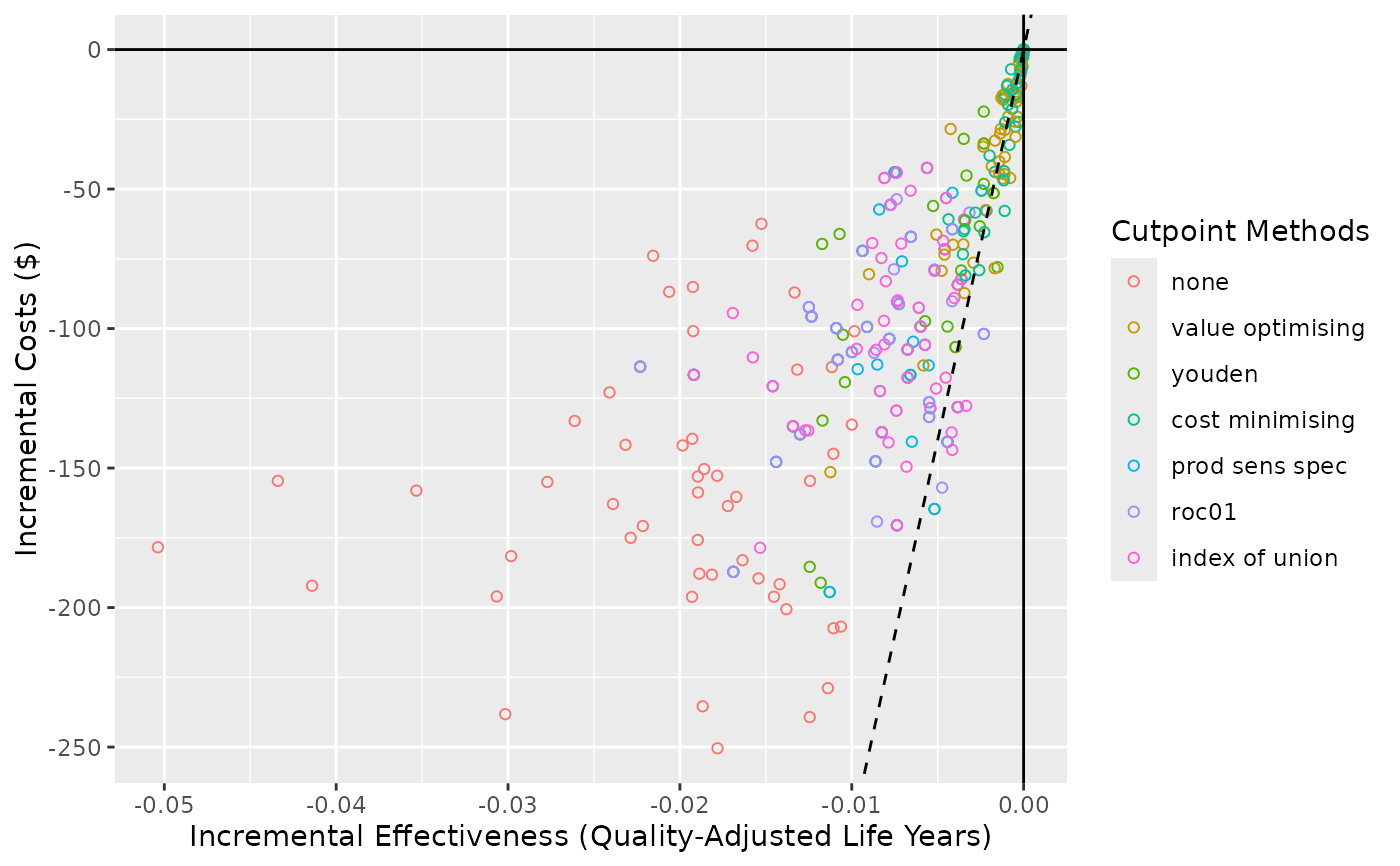
Details

This plot method works with predictNMBsim objects that are created using do_nmb_sim(). Can be used to visualise the simulations on a cost-effectiveness plot (costs vs effectiveness)

Examples

# \donttest{
get_nmb_evaluation <- get_nmb_sampler(
  qalys_lost = function() rnorm(1, 0.33, 0.03),
  wtp = 28000,
  high_risk_group_treatment_effect = function() exp(rnorm(n = 1, mean = log(0.58), sd = 0.43)),
  high_risk_group_treatment_cost = function() rnorm(n = 1, mean = 161, sd = 49)
)

sim_obj <- do_nmb_sim(
  sample_size = 200, n_sims = 50, n_valid = 10000, sim_auc = 0.7,
  event_rate = 0.1, fx_nmb_training = get_nmb_evaluation, fx_nmb_evaluation = get_nmb_evaluation
)

ce_plot(sim_obj, ref_col = "all")

# }