The tiler package provides a map tile-generator function
for creating map tile sets for use with packages such as
leaflet.
In addition to generating map tiles based on a common raster layer
source, it also handles the non-geographic edge case, producing map
tiles from arbitrary images. These map tiles, which have a “simple CRS”,
a non-geographic simple Cartesian coordinate reference system, can also
be used with leaflet when applying the simple CRS option.
Map tiles can be created from an input file with any of the following
extensions: tif, grd and nc for
spatial maps and png, jpg and bmp
for basic images.
Setup (Windows users)
Python is required as well as the gdal library for
Python. An easy recommended way for Windows users to do this in Windows
is to install OSGeo4W. It
will bring all the required Python gdal library
functionality along with it. OSGeo4W is also commonly installed along
with QGIS.
On Windows, tiler_options() is set on package load with
osgeo4w = "OSgeo4W.bat". Make sure to add the path to this
file to your system path variable. Otherwise it will not be found when
calling tile(). You can set the full path to
OSGeo4W.bat directly in your R session with
tiler_options(). However, it is recommended to add the
directory (e.g. C:/OSGeo64 or wherever
OSGeo4W.bat is located) to your system path so that you
never had to deal with it in R.
Linux and Mac users should not have to do any additional setup as
long as Python and gdal for Python are installed and
available.
Geographic map tiles
Context
For the sake of simple, expedient examples, the map tiles generated
below all use small zoom level ranges. There is also no reason to
attempt displaying the tiles here. To make these examples more
informative, each raster is loaded and plotted for context, though this
is not necessary to the tiling process. Loading the raster
package is only needed here for the print and plot calls.
The example maps packaged with tiler are not
representative of large, high resolution imagery that benefits from
tiling. These maps are very small in order to minimize package size and
ensure examples run quickly. But the tiling procedures demonstrated are
the same as would be applied to larger images.
Lastly, consider the power of your system before attempting to make a ton of tiles for large images at very high resolutions. You could find that the system could hang at any one of a number of choke points. If you are attempting to make thousands of tiles for a large, high resolution image and your system is struggling, it is recommended to (1) try making tiles for only one zoom level at a time, starting from zero and then increasing while monitoring your system resources. (2) If this is not enough, find a better system.
Basic example
Map tiles are generated with tile(). tile()
takes an input file name file for the source map and a
tiles destination path for where to save map tiles. The
only other required argument is zoom, the range of zoom
levels for the tiles. This is a string of the form,
e.g. 3:7. In this and the subsequent examples zoom levels
0-3 are used.
library(tiler)
library(raster)
tile_dir <- file.path(tempdir(), "tiles")
map <- system.file("maps/map_wgs84.tif", package = "tiler")
(r <- raster(map))
#> class      : RasterLayer
#> dimensions : 32, 71, 2272  (nrow, ncol, ncell)
#> resolution : 0.8333333, 0.8333333  (x, y)
#> extent     : -125.0208, -65.85417, 23.27083, 49.9375  (xmin, xmax, ymin, ymax)
#> crs        : +proj=longlat +datum=WGS84 +no_defs
#> source     : map_wgs84.tif
#> names      : map_wgs84
#> values     : -0.7205295, 5.545086  (min, max)
plot(r)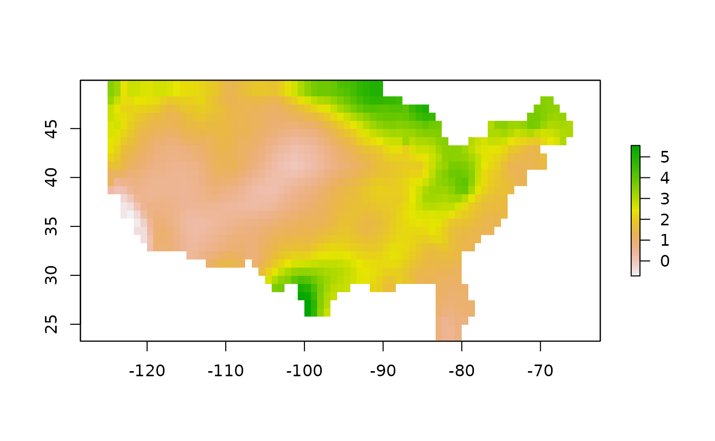
tile(map, tile_dir, "0-3")
#> Coloring raster...
#> Preparing for tiling...
#> Creating tiles. Please wait...
#> Creating tile viewer...
#> Complete.

list.files(tile_dir)
#> [1] "0"                   "1"                   "2"
#> [4] "3"                   "doc.kml"             "tilemapresource.xml"
Listing the files in tile_dir shows the top level map
tiles directories, 0-3 as expected. This is not printed in subsequent
examples since it is not going to change.
Note that these examples rendered to HTML here do not capture the
parts of the log output that result from the internal system call made
by tile(). When you run this example yourself you will see
a bit more information at the console.
Projected maps
The previous example used a map with a geospatial coordinate
reference system (CRS) but it was not projected. That map would be ready
to view with the leaflet package for example, as would the
tiles generated based on it. The next example uses a similar map that is
projected. In order to generate map tiles that can be used with
leaflet in the standard CRS, the map must be reprojected
first. Then the same map tiles are generated as before.
map <- system.file("maps/map_albers.tif", package = "tiler")
(r <- raster(map))
#> class      : RasterLayer
#> dimensions : 32, 71, 2272  (nrow, ncol, ncell)
#> resolution : 85011.74, 103363.8  (x, y)
#> extent     : -2976297, 3059536, -1577300, 1730342  (xmin, xmax, ymin, ymax)
#> crs        : +proj=aea +lat_0=37.5 +lon_0=-96 +lat_1=29.5 +lat_2=45.5 +x_0=0 +y_0=0 +datum=NAD83 +units=m +no_defs
#> source     : map_albers.tif
#> names      : map_albers
#> values     : -0.593978, 5.544724  (min, max)
plot(r)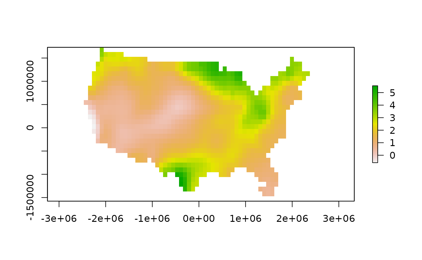
tile(map, tile_dir, "0-3")
#> Reprojecting raster...
#> Coloring raster...
#> Preparing for tiling...
#> Creating tiles. Please wait...
#> Creating tile viewer...
#> Complete.
The tiles generated this time are the same as before, that is, ready
for leaflet. tile() reprojects the raster
layer internally. This can be seen in the log output printed to the
console.
Missing CRS
If the CRS of the raster is NA, there are two options.
By default, tile() will fall back on processing the raster
layer as if it were a simple image file with no geospatial projection
information (see the next section on simple CRS/non-geographic map
tiles). These tiles are not the same as the previous sets.
map <- system.file("maps/map_albers_NA.tif", package = "tiler")
(r <- raster(map))
#> class      : RasterLayer
#> dimensions : 32, 71, 2272  (nrow, ncol, ncell)
#> resolution : 85011.74, 103363.8  (x, y)
#> extent     : -2976297, 3059536, -1577300, 1730342  (xmin, xmax, ymin, ymax)
#> crs        : NA
#> source     : map_albers_NA.tif
#> names      : map_albers_NA
#> values     : -0.593978, 5.544724  (min, max)
plot(r)
tile(map, tile_dir, "0-3")
#> Warning in .proj_check(file, crs, tmpf = tf, ...): Projection expected but is
#> missing. Continuing as non-geographic image.
#> Coloring raster...
#> Preparing for tiling...
#> Creating tiles. Please wait...
#> Creating tile viewer...
#> Complete.
This is not likely what is wanted. The other option is to force set a known CRS if it is missing from the file or was dropped for whatever reason. Now reprojection can proceed and the expected tiles are generated.
crs <- "+proj=aea +lat_1=29.5 +lat_2=45.5 +lat_0=37.5 +lon_0=-96 +x_0=0 +y_0=0 +ellps=GRS80 +datum=NAD83 +units=m +no_defs +towgs84=0,0,0"
tile(map, tile_dir, "0-3", crs)
#> Reprojecting raster...
#> Coloring raster...
#> Preparing for tiling...
#> Creating tiles. Please wait...
#> Creating tile viewer...
#> Complete.
A note on reprojection: Depending on the nature of the data in a
raster, the ... argument to tile() allows you
to pass through the method argument to
raster::projectRaster(). This is bilinear by
default for bilinear interpolation, appropriate for continuous data. It
can be set to ngb for nearest neighbor, appropriate for
discrete or categorical data. If more control is needed over the
reprojection, you should just prepare your raster file first before
using tile(). tiler is not intended to
substitute for or wrap general geospatial processing tasks that can
easily be done with other packages.
Coloring tiles
Being able to change the default color palette or specify color
breaks is important. All other optional ... arguments to
tile() are passed to raster::RGB() to provide
control over the creation of an intermediary RGB raster. Most arguments
to RGB can usually be ignored. The most useful ones are
col and colNA for the data values color
palette and the noData color, respectively. Coloring tiles
differently for the original example is as simple as the following.
map <- system.file("maps/map_wgs84.tif", package = "tiler")
pal <- colorRampPalette(c("darkblue", "lightblue"))(20)
nodata <- "tomato"
tile(map, tile_dir, "0-3", col = pal, colNA = nodata)
#> Coloring raster...
#> Preparing for tiling...
#> Creating tiles. Please wait...
#> Creating tile viewer...
#> Complete.
RGB and RGBA rasters
Multi-band rasters are supported as long as they have three or four
layers, in which case tile() assumes these represent red,
green, blue and alpha channel, respectively. Internally, single-layer
raster files are colored and converted to a three- or four-band RGB/A
raster object prior to tile generation. If file is already
such a raster, this step is simply skipped. Optional arguments like data
and noData color, break points, etc., are ignored since
this type of raster contains its own color information.
map <- system.file("maps/map_albers_rgb.tif", package = "tiler")
(r <- brick(map))
#> class      : RasterBrick
#> dimensions : 32, 71, 2272, 3  (nrow, ncol, ncell, nlayers)
#> resolution : 85011.74, 103363.8  (x, y)
#> extent     : -2976297, 3059536, -1577300, 1730342  (xmin, xmax, ymin, ymax)
#> crs        : +proj=aea +lat_0=37.5 +lon_0=-96 +lat_1=29.5 +lat_2=45.5 +x_0=0 +y_0=0 +datum=NAD83 +units=m +no_defs
#> source     : map_albers_rgb.tif
#> names      : map_albers_rgb_1, map_albers_rgb_2, map_albers_rgb_3
#> min values :                0,                0,                0
#> max values :              253,              255,              244
plot(r)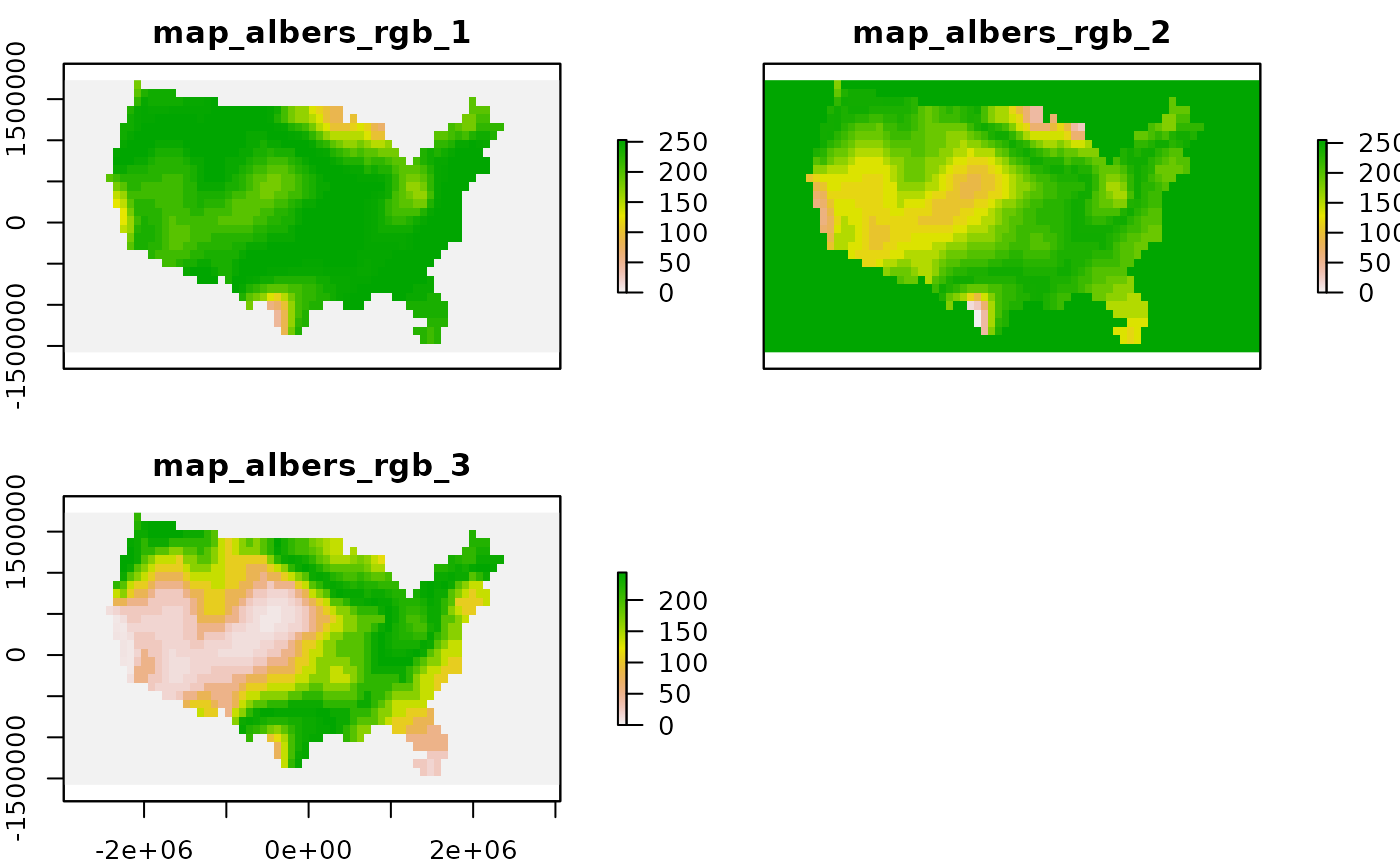
tile(map, tile_dir, "0-3")
#> Reprojecting raster...
#> Preparing for tiling...
#> Creating tiles. Please wait...
#> Creating tile viewer...
#> Complete.
Non-geographic map tiles
Almost all map tiles you encounter are for geographic maps. They have a geographic coordinate reference system (CRS). Software used to display these map tiles, such as Leaflet, is similarly focused on these kinds of map tiles. Everything is geared towards the dominant use case involving geospatial coordinate systems.
However, there are edge cases where non-geographic maps are required.
These can be maps of outer space, game board maps, etc. The base map
used to generate map tiles is usually a simple image like a
png, jpg or bmp file. The
coordinate reference system is a simple Cartesian coordinate system
based on the matrix of pixels or grid cells that represent the
image.
There is no longitude or latitude or more complex geospatial projection associated with these maps, which is why they are said to have a “simple CRS”. Simple does not necessarily mean easier to work with, however, because geospatial tools, like Leaflet for example, do not cater naturally to non-geographic coordinate systems. Using these map tiles in Leaflet is possible, but takes a bit of non-standard effort.
Basic example
One example was shown previously where a spatial map lacking critical
spatial reference information was processed as a simple image. In the
example below, this is the intent. Here, the map is a png
file. It is a previously saved plot of the Albers-projected US map used
in the earlier projected geotiff example. You can see it has a color key
legend. As a simple image, all of this will be tiled.
map <- system.file("maps/map.png", package = "tiler")
plotRGB(brick(map))
#> Warning: [rast] unknown extent
#> Warning: [rast] unknown extent
#> Warning: [rast] unknown extent
#> Warning: [rast] unknown extent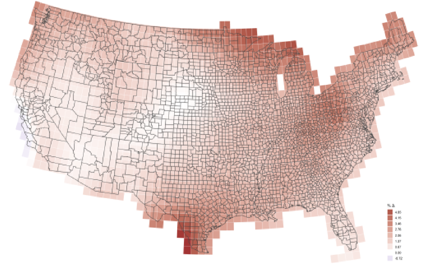
tile(map, tile_dir, "0-3")
#> Creating tiles. Please wait...
#> Creating tile viewer...
#> Complete.
The tile() function will automatically process simple
image files differently. There is no concept of projection, and coloring
tiles is irrelevant because the image file has its own coloring already.
Map tiles generated from regular image files can be used with
leaflet if done properly. The generated tiles have a simple
CRS that is based on the pixel dimensions of the image file. If you were
to use these tiles in leaflet for example and you wanted to
overlay map markers, you would have to first georeference your locations
of interest based on the matrix rows and columns of the image. This is
outside the scope of tiler. See the Leaflet JS and
leaflet package documentation for details on using simple
CRS/non-geographic tiles.
Using a png file is recommended for quality and file
size. jpg may yield a lower quality result, while a large,
high resolution bmp file may have an enormous file size
compared to png.
jpg and bmp are optionally
supported by tiler. This means they are not installed and
imported with tiler. It is assumed the user will provide
png images. If using jpg or bmp
and the packages jpeg or bmp are not
installed, respectively, tile() will print a message to the
console notifying of the required package installations.
Additional arguments
Other arguments to tile() include format,
resume, viewer and georef.
format is either xyz (default) or
tms. gdal2tiles generates TMS tiles, but XYZ
may be more familiar. Tile format only applies to geographic maps. All
simple image-based tiles are XYZ format. If setting
format = "tms" you may need to do something similar in your
Leaflet JavaScript or leaflet package R code for tiles to
display with the proper orientation.
resume = TRUE simply avoids overwriting tiles by picking
up where you left off without changing your set zoom levels and output
path.
viewer = TRUE creates preview.html adjacent
to the tiles directory for previewing tiles in the browser
using Leaflet. georef = TRUE adds mouse click feedback to
the Leaflet widget. Map markers with matrix index coordinate labels
appear on mouse click to assist with georeferencing. georef
only applies to non-geographic tiles. This allows for interactive
georeferencing of pixels in the image.
Finally, ... can pass along some additional arguments.
See help documentation for details.
Serving map tiles
Map tiles must be served online to be of much use. Serving map tiles
is not the purpose of tiler but using your GitHub account
is an easy way to do this. Create a GitHub repository, enable GitHub
pages for the repository in the repository settings. If the repository
is exclusively for serving your map tiles, just set the master branch as
the source for your GitHub pages. After committing and pushing your
tiles to GitHub, you can access them using a URL of the form
https://<your account name>.github.io/maptiles/tiles/{z}/{x}/{y}.png
if you store your tiles in a folder named tiles in a
repository named maptiles for example.
Here are some examples
of non-geographic tile sets hosted on GitHub using Star Trek galaxy
maps generated with tiler and here they are used in Leaflet
maps.
Leaflet examples using remotely hosted tiles
The following two examples use Leaflet to display interactive maps.
The maps use remotely hosted map tiles that were created with
tiler.
Geographic provider tiles based on the low resolution example map
included in tiler of the 48 contiguous US states. These map
tiles were originally generated with the following code
file <- system.file("maps/map_wgs84.tif", package = "tiler")
tile(file, "tiles", "0-7")
and are hosted here.
library(leaflet)
tiles <- "https://leonawicz.github.io/tiles/us48lr/tiles/{z}/{x}/{y}.png"
leaflet(
  options = leafletOptions(minZoom = 0, maxZoom = 7), width = "100%") %>%
  addTiles(tiles, options = tileOptions(opacity = 0.8)) %>% setView(-100, 40, 3)
Non-geographic provider tiles based on a Star Trek fictional galaxy map. These map tiles were generated with
tile("st2.png", "tiles", "0-7")and are hosted here,
including the source file st2.png.
tiles <- "https://leonawicz.github.io/tiles/st2/tiles/{z}/{x}/{y}.png"
leaflet(
  options = leafletOptions(
    crs = leafletCRS("L.CRS.Simple"), minZoom = 0, maxZoom = 7, attributionControl = FALSE), width = "100%") %>%
  addTiles(tiles) %>% setView(71, -60, 3)
*Note: These hosted tiles were made when tiler made
XYZ-format tiles. It now strictly makes TMS tiles. For new tiles in
leaflet switch the end of the url from {y} to
{-y}.
Local preview
By default tile() also creates preview.html
as noted above. This can also be created or re-created directly using
tile_viewer(). In either case, as long as
preview.html exists alongside the tiles directory, it can
easily be loaded in the browser with view_tiles(). See help
documentation for details.
If you have tiles in a directory "project/tiles",
creating preview.html directly can be done as follows. The
arguments shown are just for illustration.
tile_viewer("project/tiles", "3-7") # geographic tiles
tile_viewer("project/tiles", "3-7", width = 1000, height = 1000) # non-geographic tiles
However the tile preview document is created, it can be viewed by
passing the same tiles directory to
view_tiles.
view_tiles("project/tiles")Details
The leaflet R code needed in order to use custom
non-geographic tiles like these requires setting
leafletOptions(crs = leafletCRS("L.CRS.Simple")) as well as
calling addTiles(urlTemplate = url) where url
is like the example URL shown above. Setting the focus of the map can be
a bit tricky for non-geographic map tiles based on an arbitrary image
file. It may take some trial and error to get a sense for the custom
coordinate system.
