tracerer versus Tracer demo

Richèl J.C. Bilderbeek

2024-11-27

tracerer: ‘Tracer for R’ is an R package that does the same as Tracer does, from within R.

To use tracerer, it needs to be loaded:

library(tracerer)

When loading beast2_example_output.log in Tracer, the following is displayed:

Tracer output

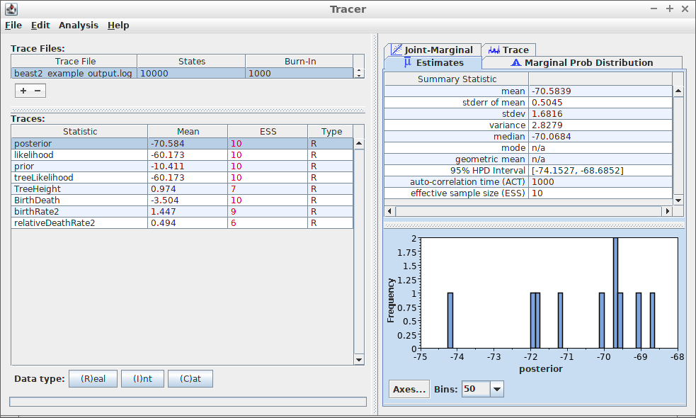
Most prominently, at the left, the effective sample sizes (ESSes) are shown.

The show the ESSes using tracerer:

estimates <- parse_beast_tracelog_file(
  get_tracerer_path("beast2_example_output.log")
)
estimates <- remove_burn_ins(estimates, burn_in_fraction = 0.1)
esses <- calc_esses(estimates, sample_interval = 1000)
table <- t(esses)
colnames(table) <- c("ESS")
knitr::kable(table)

	ESS
posterior	10
likelihood	10
prior	10
treeLikelihood	10
TreeHeight	7
BirthDeath	10
birthRate2	9
relativeDeathRate2	6

At the top-right, some measures of the variable posterior is shown. To reproduce these measures in tracerer:

sum_stats <- calc_summary_stats(
  estimates$posterior,
  sample_interval = 1000
)
table <- t(sum_stats)
colnames(table) <- c("sum_stat")
knitr::kable(table)

	sum_stat
mean	-70.58394
stderr_mean	0.5044887
stdev	1.681629
variance	2.827876
median	-69.87976
mode	n/a
geom_mean	n/a
hpd_interval_low	-74.15268
hpd_interval_high	-68.68523
act	1000
ess	10

Unlike Tracer, in tracerer all summary statistics can be obtained at once:

sum_stats <- calc_summary_stats(
  estimates,
  sample_interval = 1000
)
knitr::kable(sum_stats)

	mean	stderr_mean	stdev	variance	median	mode	geom_mean	hpd_interval_low	hpd_interval_high	act	ess
posterior	-70.5839432	0.5044887	1.6816291	2.8278764	-69.8797613	n/a	n/a	-74.1526820	-68.6852294	1000.000	10.000000
likelihood	-60.1725009	0.3964208	1.3214025	1.7461047	-60.0504225	n/a	n/a	-62.4090389	-58.7371284	1000.000	10.000000
prior	-10.4114423	0.5424505	1.8081684	3.2694729	-10.5950270	n/a	n/a	-14.1703653	-7.2820933	1000.000	10.000000
treeLikelihood	-60.1725009	0.3964208	1.3214025	1.7461047	-60.0504225	n/a	n/a	-62.4090389	-58.7371284	1000.000	10.000000
TreeHeight	0.9744748	0.1439937	0.3916244	0.1533697	0.8755907	n/a	0.91041547166058	0.4529637	1.8159958	1502.121	6.657254
BirthDeath	-3.5036870	0.5424505	1.8081684	3.2694729	-3.6872718	n/a	n/a	-7.2626100	-0.3743380	1000.000	10.000000
birthRate2	1.4470488	0.2134411	0.6713951	0.4507714	1.4118781	n/a	1.28823302868404	0.3909076	2.8041208	1122.942	8.905181
relativeDeathRate2	0.4937568	0.0650235	0.1709096	0.0292101	0.4480670	n/a	0.466468860930895	0.2496224	0.7107459	1608.296	6.217762

At the bottom-right, a histogram of the posterior estimates is shown. To reproduce these measures in tracerer:

ggplot2::ggplot(
  data = remove_burn_ins(estimates, burn_in_fraction = 0.1),
  ggplot2::aes(posterior)
) + ggplot2::geom_histogram(binwidth = 0.21) +
  ggplot2::scale_x_continuous(breaks = seq(-75, -68))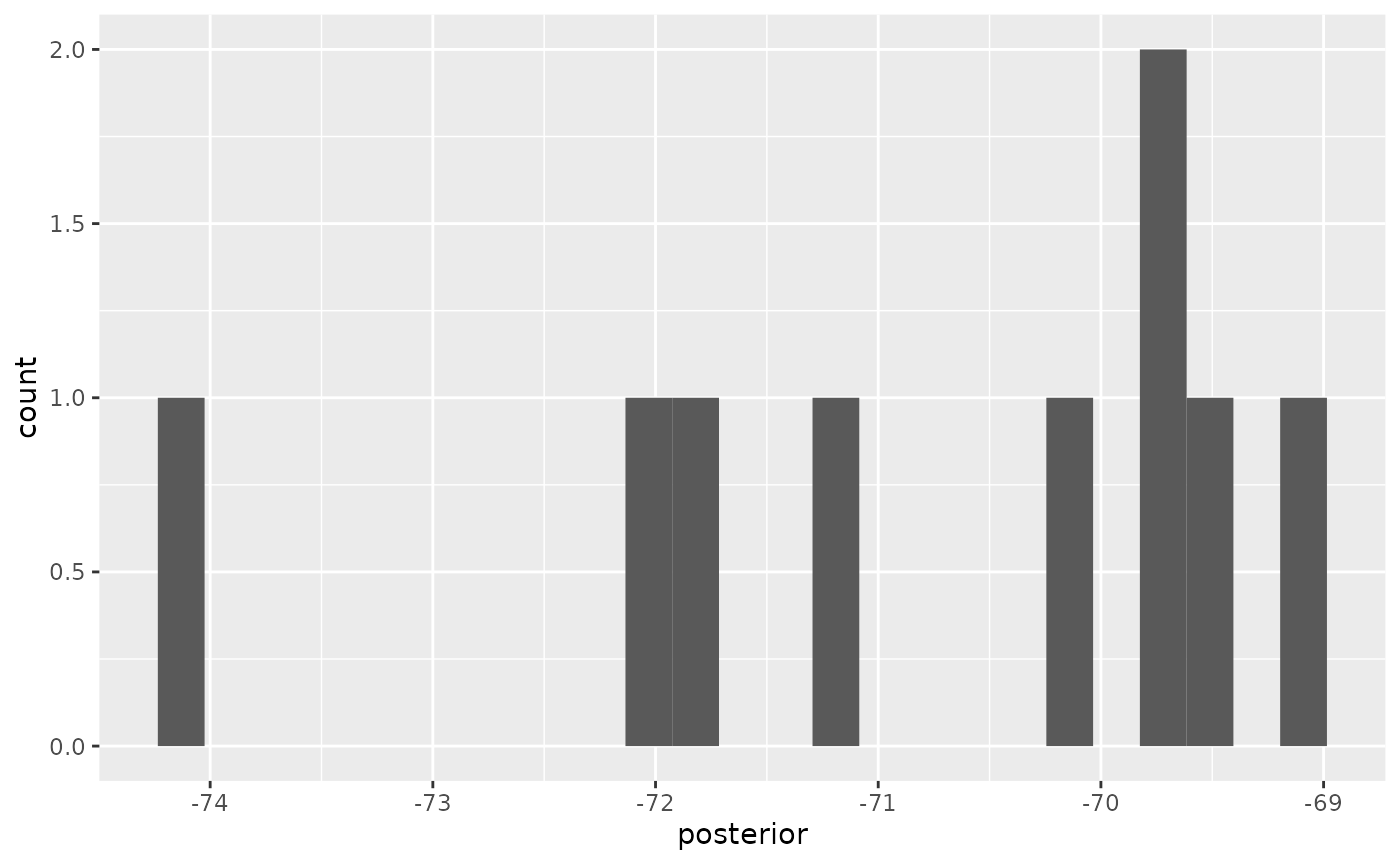

Tracer can also show the trace of each estimated variable:

Tracer shows the trace of the posterior likelihood

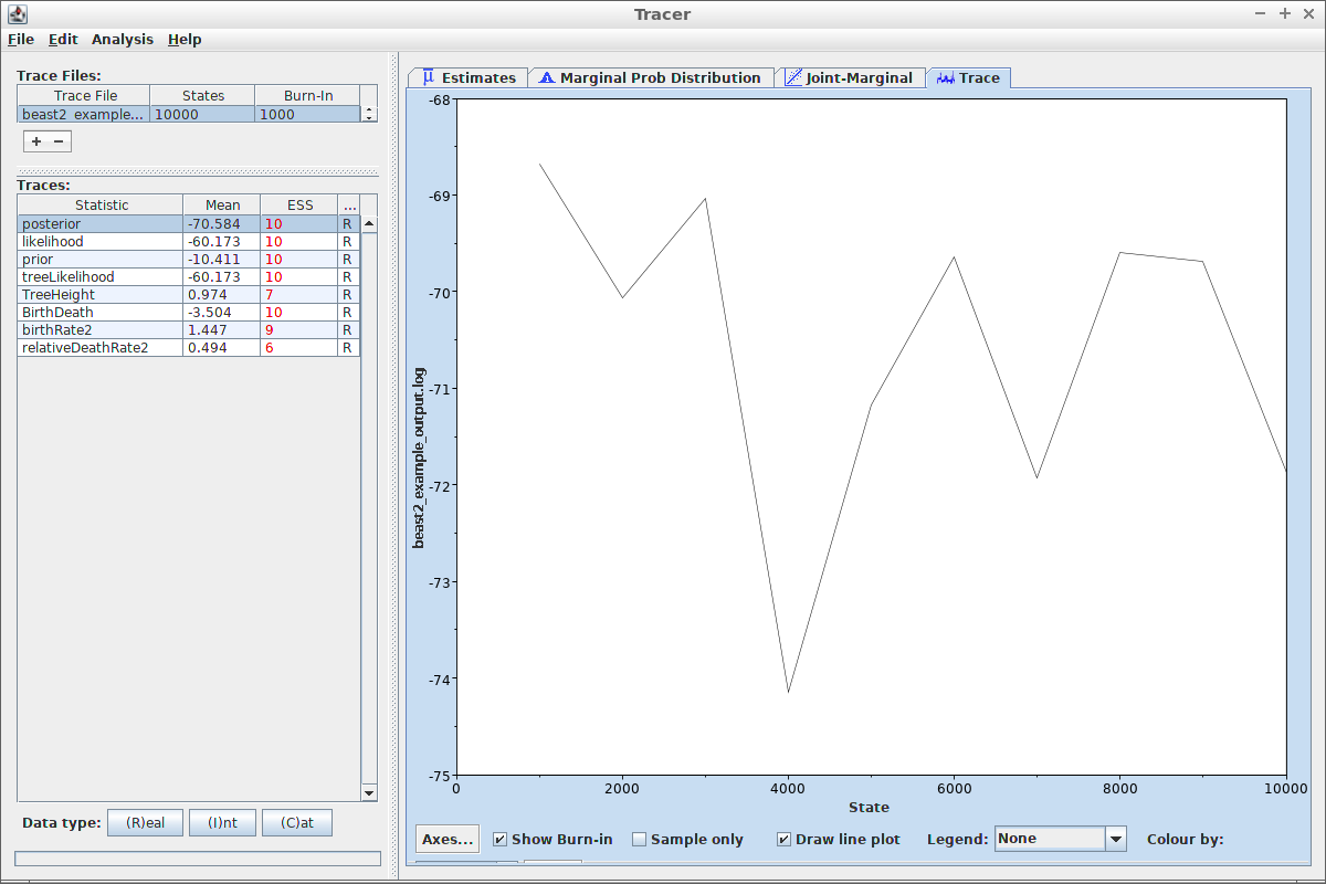
Same can be done with tracerer:

ggplot2::ggplot(
  data = remove_burn_ins(estimates, burn_in_fraction = 0.1),
  ggplot2::aes(x = Sample)
) + ggplot2::geom_line(ggplot2::aes(y = posterior))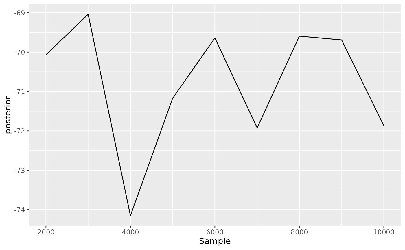

tracerer can also use part of DensiTree’s functionality. Here is beast2_example_output.trees displayed by DensiTree:

DensiTree output

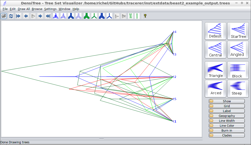
The same is achieved in tracerer with:

trees <- parse_beast_trees(
  get_tracerer_path("beast2_example_output.trees")
)
phangorn::densiTree(trees, width = 2)