Non-parametric Two-sample test

Let $x_1, x_2, \ldots, x_{n_1} \sim F$ and $y_1, y_2, \ldots, y_{n_2} \sim G$ be random samples from the distributions $F$ and $G$ , respectively. We test the null hypothesis that the two samples are generated from the same unknown distribution $\bar{F}$ , that is:

$H_0: F = G = \bar{F}$

versus the alternative hypothesis that the two distributions are different, that is

$H_1: F \not = G.$ We compute the kernel-based quadratic distance (KBQD) tests

$\mathrm{trace}_n = \frac{1}{n_1(n_1-1)}\sum_{i=1}^{n_1} \sum_{j \not=i}^{n_1} K_{\bar{F}}(\mathbf{x}_i,\mathbf{x}_j) + \frac{1}{n_2(n_2-1)}\sum_{i=1}^{n_2} \sum_{j \not=i}^{n_2} K_{\bar{F}}(\mathbf{y}_i,\mathbf{y}_j),$ and $D_{n} = \frac{1}{n_1(n_1-1)}\sum_{i=1}^{n_1} \sum_{j \not=i}^{n_2} K_{\bar{F}}(\mathbf{x}_i,\mathbf{x}_j) - \frac{2}{n_1 n_2}\sum_{i=1}^{n_1} \sum_{j =1}^{n_2} K_{\bar{F}}(\mathbf{x}_i,\mathbf{y}_j) + \frac{1}{n_2(n_2-1)}\sum_{i=1}^{n_2} \sum_{j \not=i}^{n_2} K_{\bar{F}}(\mathbf{y}_i,\mathbf{y}_j). \nonumber$ where $K_{\bar{F}}$ denotes the Normal kernel $K$ defined as

$K(\mathbf{s}, \mathbf{t}) = (2 \pi)^{-d/2} \left(\det{\mathbf{\Sigma}_h}\right)^{-\frac{1}{2}} \exp\left\{-\frac{1}{2}(\mathbf{s} - \mathbf{t})^\top \mathbf{\Sigma}_h^{-1}(\mathbf{s} - \mathbf{t})\right\},$

for every $\mathbf{s}, \mathbf{t} \in \mathbb{R}^d \times \mathbb{R}^d$ , with covariance matrix $\mathbf{\Sigma}_h = h^2 I$ and tuning parameter $h$ , centered with respect to $\bar{F} = \frac{n_1F + n_2G}{n_1 + n_2}$ . For more information about the centering of the kernel, see the documentation of the kb.test() function.

help(kb.test)

The KBQD tests exhibit high power against asymmetric alternatives that are close to the null hypothesis and with small sample size. We consider an example of this scenario. We generate the samples $x = (x_1, \ldots,x_n)$ from a standard normal distribution $N_d(0,I_d)$ and $y = (y_1, \ldots,y_n)$ from a skew-normal distribution $SN_d(0,I_d, \lambda)$ , where $d=4$ , $n=100$ and $\lambda= (0.5,\ldots,0.5)$ .

library(sn)
library(mvtnorm)
library(QuadratiK)
n <- 100
d <- 4
skewness_y <- 0.5
set.seed(2468)
x_2 <- rmvnorm(n, mean = rep(0, d))
y_2 <- rmsn(n = n, xi = 0, Omega = diag(d), alpha = rep(skewness_y, d))

The two-sample test can be performed by providing the two samples to be compared as x and y to the kb.test() function. If a value of $h$ is not provided, the function automatically performs the function select_h.

set.seed(2468)
two_test <- kb.test(x = x_2, y = y_2)
two_test

## 
##  Kernel-based quadratic distance two-sample test 
## U-statistic   Dn          Trace 
## ------------------------------------------------
## Test Statistic:   1.602379    2.048025 
## Critical Value:   1.05881     1.354038 
## H0 is rejected:   TRUE        TRUE 
## CV method:  subsampling 
## Selected tuning parameter h:  1.2

We can display the chosen optimal value of $h$ together with the power plot obtained versus the considered $h$ , for the alternatives $\delta$ in the select_h() function.

two_test@h$h_sel

## [1] 1.2

two_test@h$power.plot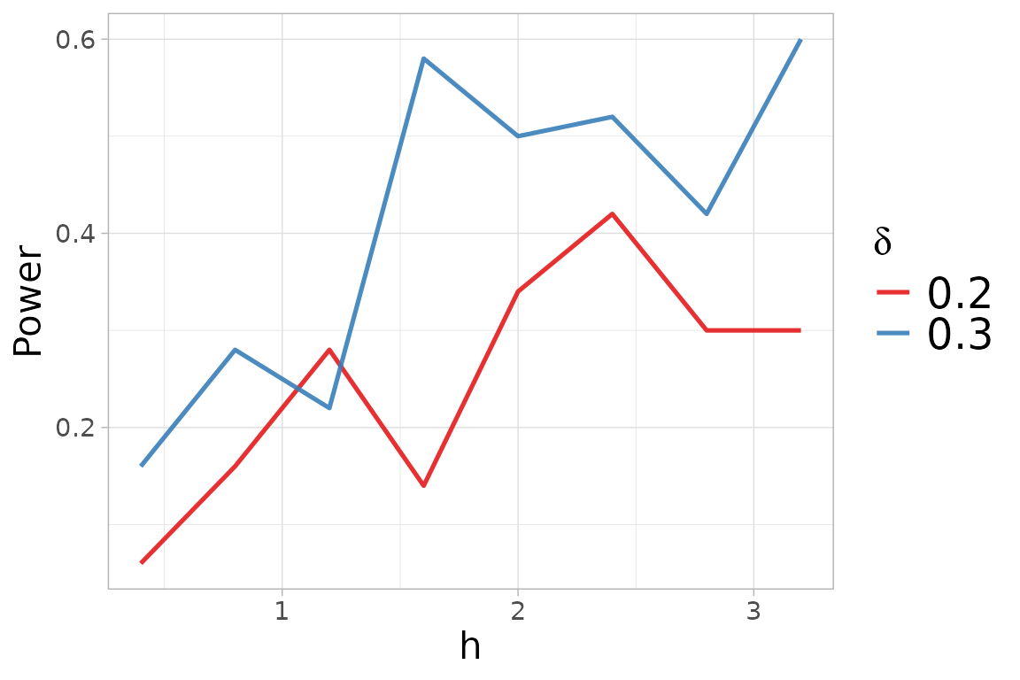

For more details visit the help documentation of the select_h() function.

help(select_h)

For the two-sample case, the summary function provides the results from the test and a list tables of the standard descriptive statistics for each variable, computed per group and overall. Additionally, it generates the qq-plots comparing the quantiles of the two groups for each variable.

summary_two <- summary(two_test)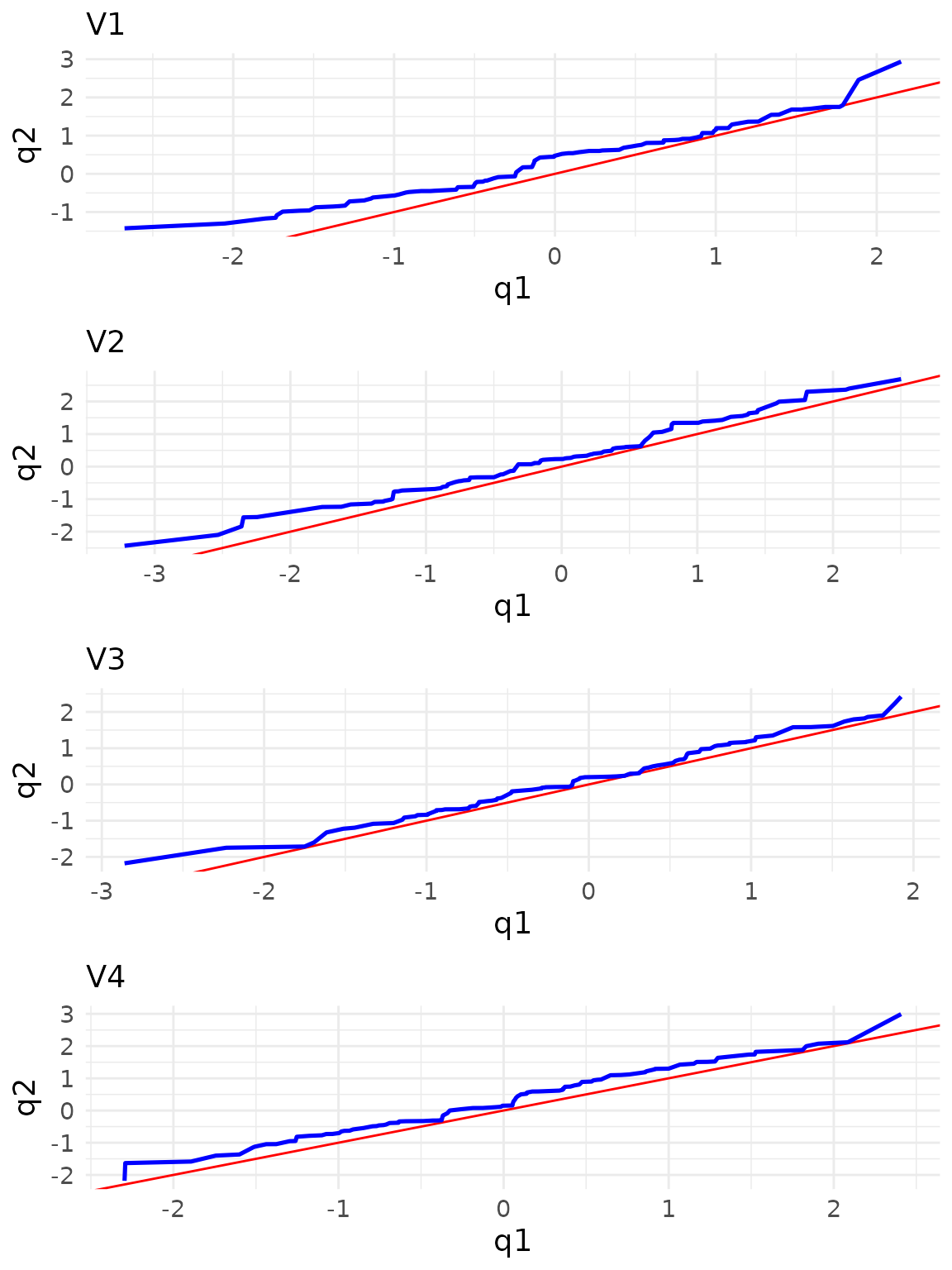

## 
##  Kernel-based quadratic distance two-sample test 
##   Statistic    Value Critical_Value Reject_H0
## 1        Dn 1.602379       1.058810      TRUE
## 2     Trace 2.048025       1.354038      TRUE

summary_two$summary_tables

## [[1]]
##             Group 1    Group 2    Overall
## mean   -0.005393522  0.3197861  0.1571963
## sd      1.039119207  0.9094193  0.9875137
## median -0.019317321  0.4448058  0.1601955
## IQR     1.562613453  1.3612937  1.4292426
## min    -2.675477796 -1.4256211 -2.6754778
## max     2.151784802  2.9375947  2.9375947
## 
## [[2]]
##            Group 1    Group 2     Overall
## mean   -0.10005083  0.1936138  0.04678149
## sd      1.10476260  1.0556439  1.08777010
## median -0.07955849  0.2235325  0.10130247
## IQR     1.48816630  1.4716179  1.41498342
## min    -3.22222061 -2.4336333 -3.22222061
## max     2.50192633  2.6879362  2.68793623
## 
## [[3]]
##             Group 1    Group 2     Overall
## mean   -0.006524772  0.1701261  0.08180065
## sd      0.958942739  0.9524916  0.95742170
## median -0.039301279  0.1887394  0.11877637
## IQR     1.329868172  1.4657107  1.40312077
## min    -2.860006689 -2.1762183 -2.86000669
## max     1.923763114  2.4237195  2.42371949
## 
## [[4]]
##            Group 1    Group 2     Overall
## mean   -0.06757686  0.2236458  0.07803449
## sd      0.98684958  0.9862135  0.99481815
## median -0.03258747  0.1097711  0.05517931
## IQR     1.30933016  1.4088334  1.39890664
## min    -2.29625537 -2.1827156 -2.29625537
## max     2.40795077  2.9929942  2.99299420

Select h

The search for the optimal value of the tuning parameter $h$ can be performed independently from the test computation using the select_h function. It requires the two samples, provided as x and y, and the considered family of alternatives.

set.seed(2468)
two_test_h <- select_h(x = x_2, y = y_2, alternative = "skewness")

The code is not evaluated since we would obtain the same results.

Note

Notice that the test statistics for two-sample testing coincide with the $k$ -sample test statistics when $k=2$ . Hence, alternatively the two sample tests can be performed providing the two samples together as x and indicating the membership to the groups with the argument y.

x_pool <- rbind(x_2, y_2)
y_memb <- rep(c(1, 2), each = n)
h <- two_test@h$h_sel
set.seed(2468)
kb.test(x = x_pool, y = y_memb, h = h)

## 
##  Kernel-based quadratic distance k-sample test 
## U-statistic   Dn          Trace 
## ------------------------------------------------
## Test Statistic:   1.602379    2.048025 
## Critical Value:   1.05881     1.354038 
## H0 is rejected:   TRUE        TRUE 
## CV method:  subsampling 
## Selected tuning parameter h:  1.2

See the k-sample test vignette for more details.

In the kb.test() function, the critical value can be computed with the subsampling, bootstrap or permutation algorithm. The default method is set to subsampling since it needs less computational time. For details on the sampling algorithm see the documentation of the kb.test() function.

For more details on the level and power performance of the considered two-sample tests, see the extensive simulation study reported in the following reference.

References

Markatou, M. and Saraceno, G. (2024). “A Unified Framework for Multivariate Two- and k-Sample Kernel-based Quadratic Distance Goodness-of-Fit Tests.”
https://doi.org/10.48550/arXiv.2407.16374

Non-parametric Two-sample test