k-sample test

Consider $k$ random samples of i.i.d. observations $\mathbf{x}^{(i)}_1, \mathbf{x}^{(i)}_{2}, \ldots, \mathbf{x}^{(i)}_{n_i} \sim F_i$, for $i = 1, \ldots, k$.

We test if the samples are generated from the same unknown distribution $\bar{F}$, that is: $$H_0: F_1 = F_2 = \ldots = F_k = \bar{F}$$ versus the alternative where two of the $k$ distributions differ, that is $$H_1: F_i \not = F_j,$$ for some $1 \le i \not = j \le k$.

Upon the construction of a matrix distance $\hat{\mathbf{D}}$, with off-diagonal elements $$\hat{D}_{ij} = \frac{1}{n_i n_j} \sum_{\ell=1}^{n_i}\sum_{r=1}^{n_j}K_{\bar{F}}(\mathbf{x}^{(i)}_\ell,\mathbf{x}^{(j)}_r), \qquad \mbox{ for }i \not= j$$ and in the diagonal $$\hat{D}_{ii} = \frac{1}{n_i (n_i -1)} \sum_{\ell=1}^{n_i}\sum_{r\not= \ell}^{n_i}K_{\bar{F}}(\mathbf{x}^{(i)}_\ell,\mathbf{x}^{(i)}_r), \qquad \mbox{ for }i = j,$$ where $K_{\bar{F}}$ denotes the Normal kernel $K$, defined as

$$K(\mathbf{s}, \mathbf{t}) = (2 \pi)^{-d/2} \left(\det{\mathbf{\Sigma}_h}\right)^{-\frac{1}{2}} \exp\left\{-\frac{1}{2}(\mathbf{s} - \mathbf{t})^\top \mathbf{\Sigma}_h^{-1}(\mathbf{s} - \mathbf{t})\right\},$$

for every $\mathbf{s}, \mathbf{t} \in \mathbb{R}^d \times \mathbb{R}^d$, with covariance matrix $\mathbf{\Sigma}_h = h^2 I$ and tuning parameter $h$, centered with respect to $$\bar{F} = \frac{n_1 \hat{F}_1 + \ldots + n_k \hat{F}_k}{n}, \quad \mbox{ with } n=\sum_{i=1}^k n_i.$$ For more information about the centering of the kernel, see the documentation of the kb.test() function.

help(kb.test) 

We compute the trace statistic $$\mathrm{trace}(\hat{\mathbf{D}}_n) = \sum_{i=1}^{k}\hat{D}_{ii}.$$ and $D_n$, derived considering all the possible pairwise comparisons in the $k$-sample null hypothesis, given as $$D_{n} = (k-1) \mathrm{trace}(\hat{\mathbf{D}}_n) - 2 \sum_{i=1}^{k}\sum_{j> i}^{k}\hat{D}_{ij}.$$

We show the usage of the kb.test() function with the following example of $k=3$ samples of bivariate observations following normal distributions with different mean vectors.

We generate three samples, with $n=50$ observations each, from a 2-dimensional Gaussian distributions with mean vectors $\mu_1 = (0, \frac{\sqrt{3}}{3})$, ${\mu}_2 = (-\frac{1}{2}, -\frac{\sqrt{3}}{6})$ and $\mu_3 = (\frac{1}{2}, -\frac{\sqrt{3}}{6})$, and the Identity matrix as covariance matrix. In this situation, the generated samples are well separated, following different Gaussian distributions, i.e. $X_1 \sim N_2(\mu_1, I)$, $X_2 \sim N_2(\mu_2, I)$ and $X_3 \sim N_2(\mu_3, I)$}. In order to perform the $k$-sample tests, we need to define the vector y which indicates the membership to groups.

library(mvtnorm)
library(QuadratiK)
library(ggplot2)
sizes <- rep(50,3)
eps <- 1
set.seed(2468)
x1 <- rmvnorm(sizes[1], mean = c(0,sqrt(3)*eps/3))
x2 <- rmvnorm(sizes[2], mean = c(-eps/2,-sqrt(3)*eps/6))
x3 <- rmvnorm(sizes[3], mean = c(eps/2,-sqrt(3)*eps/6))
x <- rbind(x1, x2, x3)
y <- as.factor(rep(c(1, 2, 3), times = sizes))

ggplot(data.frame(x = x, y = y), aes(x = x[,1], y = x[,2], color = y)) +
  geom_point(size = 2) +
  labs(title = "Generated Points", x = "X1", y = "X2") +
  theme_minimal()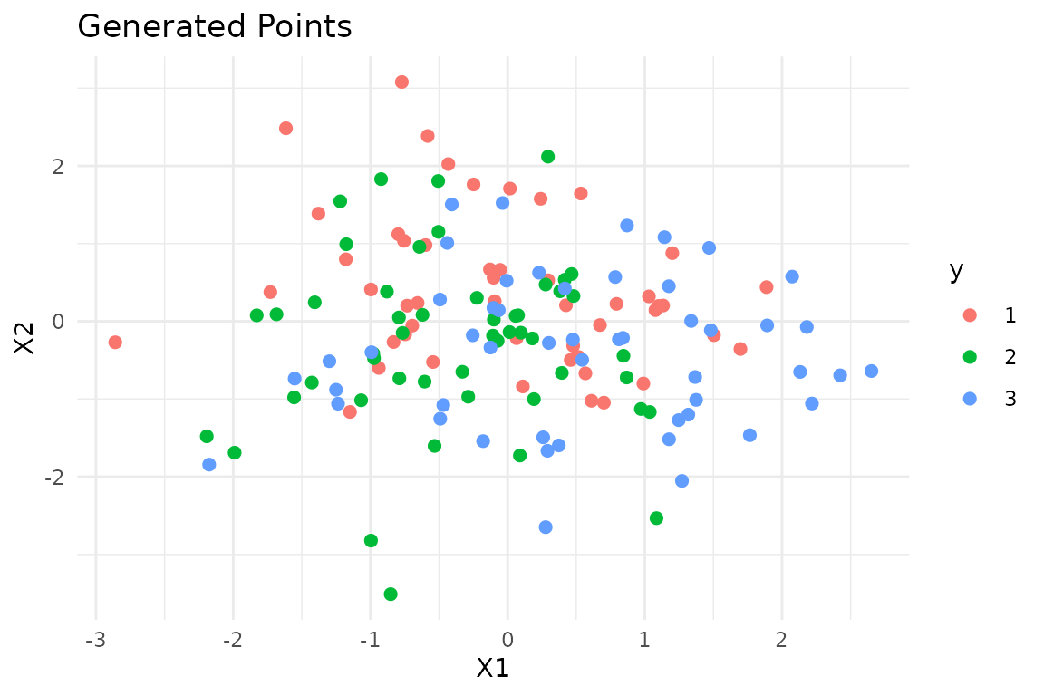

To use the kb.test() function, we need to provide the value for the tuning parameter $h$. The function select_h can be used for identifying on optimal value of $h$. This function needs the input x and y as the function kb.test, and the selection of the family of alternatives. Here we consider the location alternatives.

set.seed(2468)
h_k <- select_h(x = x, y = y, alternative = "location")

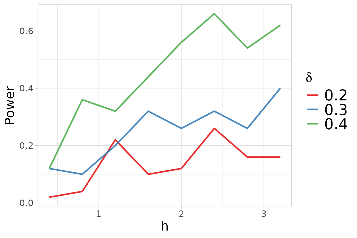
h_k$h_sel

## [1] 1.2

The select_h function has also generated a figure displaying the obtained power versus the considered $h$, for each value of alternative $\delta$ considered.

We can now perform the $k$-sample tests with the optimal value of $h$.

set.seed(2468)
k_test <- kb.test(x = x, y = y, h = h_k$h_sel)
show(k_test)

## 
##  Kernel-based quadratic distance k-sample test 
## U-statistic   Dn          Trace 
## ------------------------------------------------
## Test Statistic:   3.76127     5.552056 
## Critical Value:   1.270525    1.876836 
## H0 is rejected:   TRUE        TRUE 
## CV method:  subsampling 
## Selected tuning parameter h:  1.2

The function kb.test() returns an object of class kb.test. The show method for the kb.test object shows the computed statistics with corresponding critical values, and the logical indicating if the null hypothesis is rejected. The test correctly rejects the null hypothesis, in fact the values of the statistics are greater than the computed critical values. The package provides also the summary function which returns the results of the tests together with the standard descriptive statistics for each variable computed, overall, and with respect to the provided groups.

summary_ktest <- summary(k_test)

## 
##  Kernel-based quadratic distance k-sample test 
##   Statistic    Value Critical_Value Reject_H0
## 1        Dn 3.761270       1.270525      TRUE
## 2     Trace 5.552056       1.876836      TRUE

summary_ktest$summary_tables

## [[1]]
##            Group 1    Group 2    Group 3      Overall
## mean   -0.05208816 -0.3961768  0.5318161  0.027850399
## sd      0.96223294  0.8169982  1.1147943  1.039422979
## median -0.07433374 -0.4171737  0.4466713  0.003313025
## IQR     1.34379740  1.1499518  1.4976634  1.507024820
## min    -2.86000669 -2.1929616 -2.1754778 -2.860006689
## max     1.88750642  1.0851059  2.6517848  2.651784802
## 
## [[2]]
##           Group 1    Group 2    Group 3     Overall
## mean    0.3928294 -0.2851004 -0.4028292 -0.09836674
## sd      0.9612003  1.1243216  0.9603282  1.07079458
## median  0.2303015 -0.1667130 -0.3676814 -0.14246592
## IQR     1.1269249  1.2443774  1.3256384  1.24637078
## min    -1.1662595 -3.5108957 -2.6488286 -3.51089574
## max     3.0792766  2.1192756  1.5225887  3.07927659

Note

If a value of $h$ is not provided to kb.test(), this function performs the function select_h for automatic search of an optimal value of $h$ to use. . The following code shows its usage, but it is not executed since we would obtain the same results.

k_test_h <- kb.test(x = x, y = y)

For more details visit the help documentation of the select_h() function.

help(select_h) 

In the kb.test() function, the critical value can be computed with the subsampling, bootstrap or permutation algorithm. The default method is set to subsampling since it needs less computational time. For details on the sampling algorithm see the documentation of the kb.test() function and the following reference.

The proposed tests exhibit high power against asymmetric alternatives that are close to the null hypothesis and with small sample size, as well as in the $k \ge 3$ sample comparison, for dimension $d>2$ and all sample sizes. For more details, see the extensive simulation study reported in the following reference.

References

Markatou, M. and Saraceno, G. (2024). “A Unified Framework for Multivariate Two- and k-Sample Kernel-based Quadratic Distance Goodness-of-Fit Tests.”
https://doi.org/10.48550/arXiv.2407.16374