Oblique Random Forests

Grow or specify an oblique random forest. While the name orsf() implies that this function only works for survival forests, it can be used for classification, regression, or survival forests.

Usage

orsf(
  data,
  formula,
  control = NULL,
  weights = NULL,
  n_tree = 500,
  n_split = 5,
  n_retry = 3,
  n_thread = 0,
  mtry = NULL,
  sample_with_replacement = TRUE,
  sample_fraction = 0.632,
  leaf_min_events = 1,
  leaf_min_obs = 5,
  split_rule = NULL,
  split_min_events = 5,
  split_min_obs = 10,
  split_min_stat = NULL,
  oobag_pred_type = NULL,
  oobag_pred_horizon = NULL,
  oobag_eval_every = NULL,
  oobag_fun = NULL,
  importance = "anova",
  importance_max_pvalue = 0.01,
  group_factors = TRUE,
  tree_seeds = NULL,
  attach_data = TRUE,
  no_fit = FALSE,
  na_action = "fail",
  verbose_progress = FALSE,
  ...
)

orsf_train(object, attach_data = TRUE)

Arguments

data

a data.frame, tibble, or data.table that contains the relevant variables.

formula

(formula) Two sided formula with a single outcome. The terms on the right are names of predictor variables, and the symbol '.' may be used to indicate all variables in the data except the response. The symbol '-' may also be used to indicate removal of a predictor. Details on the response vary depending on forest type:

Classification: The response should be a single variable, and that variable should have type factor in data.
Regression: The response should be a single variable, and that variable should have typee double or integer with at least 10 unique numeric values in data.
Survival: The response should include a time variable, followed by a status variable, and may be written inside a call to Surv (see examples).

control

(orsf_control) An object returned from one of the orsf_control functions: orsf_control_survival, orsf_control_classification, and orsf_control_regression. If NULL (the default) will use an accelerated control, which is the fastest available option. For survival and classification, this is Cox and Logistic regression with 1 iteration, and for regression it is ordinary least squares.

weights

(numeric vector) Optional. If given, this input should have length equal to nrow(data) for complete or imputed data and should have length equal to nrow(na.omit(data)) if na_action is "omit". As the weights vector is used to count observations and events prior to growing a node for a tree, orsf() scales weights so that sum(weights) == nrow(data). This helps to make tree depth consistent between weighted and un-weighted fits.

n_tree

(integer) the number of trees to grow. Default is n_tree = 500.

n_split

(integer) the number of cut-points assessed when splitting a node in decision trees. Default is n_split = 5.

n_retry

(integer) when a node is splittable, but the current linear combination of inputs is unable to provide a valid split, orsf will try again with a new linear combination based on a different set of randomly selected predictors, up to n_retry times. Default is n_retry = 3. Set n_retry = 0 to prevent any retries.

n_thread

(integer) number of threads to use while growing trees, computing predictions, and computing importance. Default is 0, which allows a suitable number of threads to be used based on availability.

mtry

(integer) Number of predictors randomly included as candidates for splitting a node. The default is the smallest integer greater than the square root of the number of total predictors, i.e., mtry = ceiling(sqrt(number of predictors))

sample_with_replacement

(logical) If TRUE (the default), observations are sampled with replacement when an in-bag sample is created for a decision tree. If FALSE, observations are sampled without replacement and each tree will have an in-bag sample containing sample_fraction% of the original sample.

sample_fraction

(double) the proportion of observations that each trees' in-bag sample will contain, relative to the number of rows in data. Only used if sample_with_replacement is FALSE. Default value is 0.632.

leaf_min_events

(integer) This input is only relevant for survival analysis, and specifies the minimum number of events in a leaf node. Default is leaf_min_events = 1

leaf_min_obs

(integer) minimum number of observations in a leaf node. Default is leaf_min_obs = 5.

split_rule

(character) how to assess the quality of a potential splitting rule for a node. Valid options for survival are:

'logrank' : a log-rank test statistic (default).
'cstat' : Harrell's concordance statistic.

For classification, valid options are:

'gini' : gini impurity (default)
'cstat' : area underneath the ROC curve (AUC-ROC)

For regression, valid options are:

'variance' : variance reduction (default)

split_min_events

(integer) minimum number of events required in a node to consider splitting it. Default is split_min_events = 5. This input is only relevant for survival trees.

split_min_obs

(integer) minimum number of observations required in a node to consider splitting it. Default is split_min_obs = 10.

split_min_stat

(double) minimum test statistic required to split a node. If no splits are found with a statistic exceeding split_min_stat, the given node either becomes a leaf or a retry occurs (up to n_retry retries). Defaults are

3.84 if split_rule = 'logrank'
0.55 if split_rule = 'cstat' (see first note below)
0.00 if split_rule = 'gini' (see second note below)
0.00 if split_rule = 'variance'

Note 1 For C-statistic splitting, if C is < 0.50, we consider the statistic value to be 1 - C to allow for good 'anti-predictive' splits. So, if a C-statistic is initially computed as 0.1, it will be considered as 1 - 0.10 = 0.90.

Note 2 For Gini impurity, a value of 0 and 1 usually indicate the best and worst possible scores, respectively. To make things simple and to avoid introducing a split_max_stat input, we flip the values of Gini impurity so that 1 and 0 indicate the best and worst possible scores, respectively.

oobag_pred_type

(character) The type of out-of-bag predictions to compute while fitting the ensemble. Valid options for any tree type:

'none' : don't compute out-of-bag predictions
'leaf' : the ID of the predicted leaf is returned for each tree

Valid options for survival:

'risk' : probability of event occurring at or before oobag_pred_horizon (default).
'surv' : 1 - risk.
'chf' : cumulative hazard function at oobag_pred_horizon.
'mort' : mortality, i.e., the number of events expected if all observations in the training data were identical to a given observation.

Valid options for classification:

'prob' : probability of each class (default)
'class' : class (i.e., which.max(prob))

Valid options for regression:

'mean' : mean value (default)

oobag_pred_horizon

(numeric) A numeric value indicating what time should be used for out-of-bag predictions. Default is the median of the observed times, i.e., oobag_pred_horizon = median(time). This input is only relevant for survival trees that have prediction type of 'risk', 'surv', or 'chf'.

oobag_eval_every

(integer) The out-of-bag performance of the ensemble will be checked every oobag_eval_every trees. So, if oobag_eval_every = 10, then out-of-bag performance is checked after growing the 10th tree, the 20th tree, and so on. Default is oobag_eval_every = n_tree.

oobag_fun

(function) to be used for evaluating out-of-bag prediction accuracy every oobag_eval_every trees. When oobag_fun = NULL (the default), the evaluation statistic is selected based on tree type

survival: Harrell's C-statistic (1982)
classification: Area underneath the ROC curve (AUC-ROC)
regression: Traditional prediction R-squared

if you use your own oobag_fun note the following:

oobag_fun should have three inputs: y_mat, w_vec, and s_vec
For survival trees, y_mat should be a two column matrix with first column named 'time' and second named 'status'. For classification trees, y_mat should be a matrix with number of columns = number of distinct classes in the outcome. For regression, y_mat should be a matrix with one column.
s_vec is a numeric vector containing predictions
oobag_fun should return a numeric output of length 1

For more details, see the out-of-bag vignette.

importance

(character) Indicate method for variable importance:

'none': no variable importance is computed.
'anova': compute analysis of variance (ANOVA) importance
'negate': compute negation importance
'permute': compute permutation importance

For details on these methods, see orsf_vi.

importance_max_pvalue

(double) Only relevant if importance is "anova". The maximum p-value that will register as a positive case when counting the number of times a variable was found to be 'significant' during tree growth. Default is 0.01, as recommended by Menze et al.

group_factors

(logical) Only relevant if variable importance is being estimated. if TRUE, the importance of factor variables will be reported overall by aggregating the importance of individual levels of the factor. If FALSE, the importance of individual factor levels will be returned.

tree_seeds

(integer vector) Optional. if specified, random seeds will be set using the values in tree_seeds[i] before growing tree i. Two forests grown with the same number of trees and the same seeds will have the exact same out-of-bag samples, making out-of-bag error estimates of the forests more comparable. If NULL (the default), seeds are picked at random.

attach_data

(logical) if TRUE, a copy of the training data will be attached to the output. This is required if you plan on using functions like orsf_pd_oob or orsf_summarize_uni to interpret the forest using its training data. Default is TRUE.

no_fit

(logical) if TRUE, model fitting steps are defined and saved, but training is not initiated. The object returned can be directly submitted to orsf_train() so long as attach_data is TRUE.

na_action

(character) what should happen when data contains missing values (i.e., NA values). Valid options are:

'fail' : an error is thrown if data contains NA values
'omit' : rows in data with incomplete data will be dropped
'impute_meanmode' : missing values for continuous and categorical variables in data will be imputed using the mean and mode, respectively.

verbose_progress

(logical) if TRUE, progress messages are printed in the console. If FALSE (the default), nothing is printed.

...

Further arguments passed to or from other methods (not currently used).

object

an untrained 'aorsf' object, created by setting no_fit = TRUE in orsf().

Value

an obliqueForest object

Details

Why isn't this function called orf()? In its earlier versions, the aorsf package was exclusively for oblique random survival forests.

formula for survival oblique RFs:

The response in formula can be a survival object as returned by the Surv function, but can also just be the time and status variables. I.e., Surv(time, status) ~ . works and time + status ~ . works
The response can also be a survival object stored in data. For example, y ~ . is a valid formula if data$y inherits from the Surv class.

mtry:

The mtry parameter may be temporarily reduced to ensure that linear models used to find combinations of predictors remain stable. This occurs because coefficients in linear model fitting algorithms may become infinite if the number of predictors exceeds the number of observations.

oobag_fun:

If oobag_fun is specified, it will be used in to compute negation importance or permutation importance, but it will not have any role for ANOVA importance.

n_thread:

If an R function is to be called from C++ (i.e., user-supplied function to compute out-of-bag error or identify linear combinations of variables), n_thread will automatically be set to 1 because attempting to run R functions in multiple threads will cause the R session to crash.

What is an oblique decision tree?

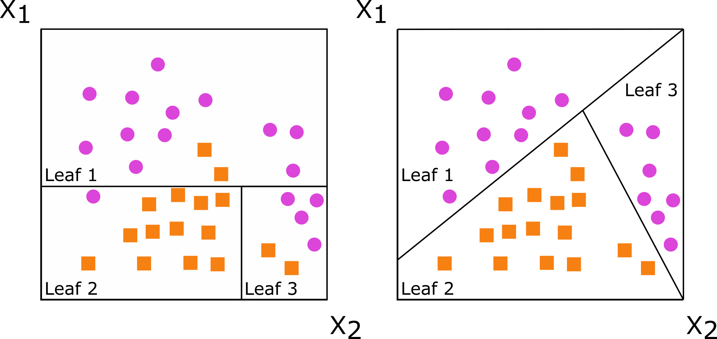
Decision trees are developed by splitting a set of training data into two new subsets, with the goal of having more similarity within the new subsets than between them. This splitting process is repeated on the resulting subsets of data until a stopping criterion is met. When the new subsets of data are formed based on a single predictor, the decision tree is said to be axis-based because the splits of the data appear perpendicular to the axis of the predictor. When linear combinations of variables are used instead of a single variable, the tree is oblique because the splits of the data are neither parallel nor at a right angle to the axis

Figure : Decision trees for classification with axis-based splitting (left) and oblique splitting (right). Cases are orange squares; controls are purple circles. Both trees partition the predictor space defined by variables X1 and X2, but the oblique splits do a better job of separating the two classes.

What is a random forest?

Random forests are collections of de-correlated decision trees. Predictions from each tree are aggregated to make an ensemble prediction for the forest. For more details, see Breiman at el, 2001.

Training, out-of-bag error, and testing

In random forests, each tree is grown with a bootstrapped version of the training set. Because bootstrap samples are selected with replacement, each bootstrapped training set contains about two-thirds of instances in the original training set. The 'out-of-bag' data are instances that are not in the bootstrapped training set. Each tree in the random forest can make predictions for its out-of-bag data, and the out-of-bag predictions can be aggregated to make an ensemble out-of-bag prediction. Since the out-of-bag data are not used to grow the tree, the accuracy of the ensemble out-of-bag predictions approximate the generalization error of the random forest. Generalization error refers to the error of a random forest's predictions when it is applied to predict outcomes for data that were not used to train it, i.e., testing data.

Examples

library(aorsf)
library(magrittr) # for %>%
#> 
#> Attaching package: 'magrittr'
#> The following objects are masked from 'package:testthat':
#> 
#>     equals, is_less_than, not

orsf() is the entry-point of the aorsf package. It can be used to fit classification, regression, and survival forests.

For classification, we fit an oblique RF to predict penguin species using penguin data from the magnificent palmerpenguins R package

# An oblique classification RF
penguin_fit <- orsf(data = penguins_orsf,
                    n_tree = 5, 
                    formula = species ~ .)

penguin_fit
#> ---------- Oblique random classification forest
#> 
#>      Linear combinations: Accelerated Logistic regression
#>           N observations: 333
#>                N classes: 3
#>                  N trees: 5
#>       N predictors total: 7
#>    N predictors per node: 3
#>  Average leaves per tree: 4.8
#> Min observations in leaf: 5
#>           OOB stat value: 0.98
#>            OOB stat type: AUC-ROC
#>      Variable importance: anova
#> 
#> -----------------------------------------

For regression, we use the same data but predict bill length of penguins:

# An oblique regression RF
bill_fit <- orsf(data = penguins_orsf, 
                 n_tree = 5, 
                 formula = bill_length_mm ~ .)

bill_fit
#> ---------- Oblique random regression forest
#> 
#>      Linear combinations: Accelerated Linear regression
#>           N observations: 333
#>                  N trees: 5
#>       N predictors total: 7
#>    N predictors per node: 3
#>  Average leaves per tree: 50.4
#> Min observations in leaf: 5
#>           OOB stat value: 0.74
#>            OOB stat type: RSQ
#>      Variable importance: anova
#> 
#> -----------------------------------------

My personal favorite is the oblique survival RF with accelerated Cox regression because it was the first type of oblique RF that aorsf provided (see ArXiv paper; the paper is also published in Journal of Computational and Graphical Statistics but is not publicly available there). Here, we use it to predict mortality risk following diagnosis of primary biliary cirrhosis:

# An oblique survival RF
pbc_fit <- orsf(data = pbc_orsf, 
                n_tree = 5,
                formula = Surv(time, status) ~ . - id)

pbc_fit
#> ---------- Oblique random survival forest
#> 
#>      Linear combinations: Accelerated Cox regression
#>           N observations: 276
#>                 N events: 111
#>                  N trees: 5
#>       N predictors total: 17
#>    N predictors per node: 5
#>  Average leaves per tree: 19.6
#> Min observations in leaf: 5
#>       Min events in leaf: 1
#>           OOB stat value: 0.78
#>            OOB stat type: Harrell's C-index
#>      Variable importance: anova
#> 
#> -----------------------------------------

More than one way to grow a forest

You can use orsf(no_fit = TRUE) to make a specification to grow a forest instead of a fitted forest.

orsf_spec <- orsf(pbc_orsf, 
                  formula = time + status ~ . - id,
                  no_fit = TRUE)

orsf_spec
#> Untrained oblique random survival forest
#> 
#>      Linear combinations: Accelerated Cox regression
#>           N observations: 276
#>                 N events: 111
#>                  N trees: 500
#>       N predictors total: 17
#>    N predictors per node: 5
#>  Average leaves per tree: 0
#> Min observations in leaf: 5
#>       Min events in leaf: 1
#>           OOB stat value: none
#>            OOB stat type: Harrell's C-index
#>      Variable importance: anova
#> 
#> -----------------------------------------

Why would you do this? Two reasons:

For very computational tasks, you may want to check how long it will take to fit the forest before you commit to it:


orsf_spec %>% 
 orsf_update(n_tree = 10000) %>%
 orsf_time_to_train()
#> Time difference of 2.029378 secs

If fitting multiple forests, use the blueprint along with orsf_train() and orsf_update() to simplify your code:


orsf_fit <- orsf_train(orsf_spec)
orsf_fit_10 <- orsf_update(orsf_fit, leaf_min_obs = 10)
orsf_fit_20 <- orsf_update(orsf_fit, leaf_min_obs = 20)

orsf_fit$leaf_min_obs
#> [1] 5
orsf_fit_10$leaf_min_obs
#> [1] 10
orsf_fit_20$leaf_min_obs
#> [1] 20

tidymodels

tidymodels includes support for aorsf as a computational engine:


library(tidymodels)
library(censored)
library(yardstick)

pbc_tidy <- pbc_orsf %>% 
 mutate(event_time = Surv(time, status), .before = 1) %>% 
 select(-c(id, time, status)) %>% 
 as_tibble()

split  <- initial_split(pbc_tidy)

orsf_spec <- rand_forest() %>% 
 set_engine("aorsf") %>% 
 set_mode("censored regression")

orsf_fit <- fit(orsf_spec, 
                formula = event_time ~ ., 
                data = training(split))

Prediction with aorsf models at different times is also supported:


time_points <- seq(500, 3000, by = 500)

test_pred <- augment(orsf_fit, 
                     new_data = testing(split), 
                     eval_time = time_points)

brier_scores <- test_pred %>% 
  brier_survival(truth = event_time, .pred)

brier_scores
#> # A tibble: 6 x 4
#>   .metric        .estimator .eval_time .estimate
#>   <chr>          <chr>           <dbl>     <dbl>
#> 1 brier_survival standard          500    0.0515
#> 2 brier_survival standard         1000    0.0988
#> 3 brier_survival standard         1500    0.0830
#> 4 brier_survival standard         2000    0.0667
#> 5 brier_survival standard         2500    0.102 
#> 6 brier_survival standard         3000    0.141

roc_scores <- test_pred %>% 
  roc_auc_survival(truth = event_time, .pred)

roc_scores
#> # A tibble: 6 x 4
#>   .metric          .estimator .eval_time .estimate
#>   <chr>            <chr>           <dbl>     <dbl>
#> 1 roc_auc_survival standard          500     0.977
#> 2 roc_auc_survival standard         1000     0.954
#> 3 roc_auc_survival standard         1500     0.965
#> 4 roc_auc_survival standard         2000     0.975
#> 5 roc_auc_survival standard         2500     0.974
#> 6 roc_auc_survival standard         3000     0.955

References

Harrell, E F, Califf, M R, Pryor, B D, Lee, L K, Rosati, A R (1982). "Evaluating the yield of medical tests." Jama, 247(18), 2543-2546.
Breiman, Leo (2001). "Random Forests." Machine Learning, 45(1), 5-32. ISSN 1573-0565.
Ishwaran H, Kogalur UB, Blackstone EH, Lauer MS (2008). "Random survival forests." The Annals of Applied Statistics, 2(3).
Menze, H B, Kelm, Michael B, Splitthoff, N D, Koethe, Ullrich, Hamprecht, A F (2011). "On oblique random forests." In Machine Learning and Knowledge Discovery in Databases: European Conference, ECML PKDD 2011, Athens, Greece, September 5-9, 2011, Proceedings, Part II 22, 453-469. Springer.
Jaeger BC, Long DL, Long DM, Sims M, Szychowski JM, Min Y, Mcclure LA, Howard G, Simon N (2019). "Oblique random survival forests." The Annals of Applied Statistics, 13(3).
Jaeger BC, Welden S, Lenoir K, Speiser JL, Segar MW, Pandey A, Pajewski NM (2023). "Accelerated and interpretable oblique random survival forests." Journal of Computational and Graphical Statistics, 1-16.