Partial dependence (PD)
Partial dependence (PD) shows the expected prediction from a model as a function of a single predictor or multiple predictors. The expectation is marginalized over the values of all other predictors, giving something like a multivariable adjusted estimate of the model’s prediction.
You can compute PD and individual conditional expectation (ICE) in three ways:
using in-bag predictions for the training data. In-bag PD indicates relationships that the model has learned during training. This is helpful if your goal is to interpret the model.
using out-of-bag predictions for the training data. Out-of-bag PD indicates relationships that the model has learned during training but using the out-of-bag data simulates application of the model to new data. This is helpful if you want to test your model’s reliability or fairness in new data but you don’t have access to a large testing set.
using predictions for a new set of data. New data PD shows how the model predicts outcomes for observations it has not seen. This is helpful if you want to test your model’s reliability or fairness.
Classification
Begin by fitting an oblique classification random forest:
set.seed(329)

index_train <- sample(nrow(penguins_orsf), 150)

penguins_orsf_train <- penguins_orsf[index_train, ]
penguins_orsf_test <- penguins_orsf[-index_train, ]

fit_clsf <- orsf(data = penguins_orsf_train,
                 formula = species ~ .)
Compute PD using out-of-bag data for
flipper_length_mm = c(190, 210).
pred_spec <- list(flipper_length_mm = c(190, 210))

pd_oob <- orsf_pd_oob(fit_clsf, pred_spec = pred_spec)

pd_oob
#> Key: <class>
#>        class flipper_length_mm      mean         lwr       medn       upr
#>       <fctr>             <num>     <num>       <num>      <num>     <num>
#> 1:    Adelie               190 0.6182417 0.206899034 0.75537171 0.9796439
#> 2:    Adelie               210 0.4348386 0.019519733 0.56802082 0.8620694
#> 3: Chinstrap               190 0.2114905 0.018420139 0.15561560 0.7174734
#> 4: Chinstrap               210 0.1806274 0.020409141 0.09928047 0.6990198
#> 5:    Gentoo               190 0.1702678 0.001281382 0.02830728 0.5733438
#> 6:    Gentoo               210 0.3845340 0.072260715 0.20258335 0.9519486
Note that predicted probabilities are returned for each class and
probabilities in the mean column sum to 1 if you take the
sum over each class at a specific value of the pred_spec
variables. For example,
sum(pd_oob[flipper_length_mm == 190, mean])
#> [1] 1
But this isn’t the case for the median predicted probability!
sum(pd_oob[flipper_length_mm == 190, medn])
#> [1] 0.9392946
Regression
Begin by fitting an oblique regression random forest:
set.seed(329)

index_train <- sample(nrow(penguins_orsf), 150)

penguins_orsf_train <- penguins_orsf[index_train, ]
penguins_orsf_test <- penguins_orsf[-index_train, ]

fit_regr <- orsf(data = penguins_orsf_train,
                 formula = bill_length_mm ~ .)
Compute PD using new data for
flipper_length_mm = c(190, 210).
pred_spec <- list(flipper_length_mm = c(190, 210))

pd_new <- orsf_pd_new(fit_regr,
                      pred_spec = pred_spec,
                      new_data = penguins_orsf_test)

pd_new
#>    flipper_length_mm     mean      lwr     medn      upr
#>                <num>    <num>    <num>    <num>    <num>
#> 1:               190 42.96571 37.09805 43.69769 48.72301
#> 2:               210 45.66012 40.50693 46.31577 51.65163
You can also let pred_spec_auto pick reasonable values
like so:
pred_spec = pred_spec_auto(species, island, body_mass_g)

pd_new <- orsf_pd_new(fit_regr,
                      pred_spec = pred_spec,
                      new_data = penguins_orsf_test)

pd_new
#>       species    island body_mass_g     mean      lwr     medn      upr
#>        <fctr>    <fctr>       <num>    <num>    <num>    <num>    <num>
#>  1:    Adelie    Biscoe        3200 40.31374 37.24373 40.31967 44.22824
#>  2: Chinstrap    Biscoe        3200 45.10582 42.63342 45.10859 47.60119
#>  3:    Gentoo    Biscoe        3200 42.81649 40.19221 42.55664 46.84035
#>  4:    Adelie     Dream        3200 40.16219 36.95895 40.34633 43.90681
#>  5: Chinstrap     Dream        3200 46.21778 43.53954 45.90929 49.19173
#>  6:    Gentoo     Dream        3200 42.60465 39.89647 42.63520 46.28769
#>  7:    Adelie Torgersen        3200 39.91652 36.80227 39.79806 43.68842
#>  8: Chinstrap Torgersen        3200 44.27807 41.95470 44.40742 46.68848
#>  9:    Gentoo Torgersen        3200 42.09510 39.49863 41.80049 45.81833
#> 10:    Adelie    Biscoe        3550 40.77971 38.04027 40.59561 44.57505
#> 11: Chinstrap    Biscoe        3550 45.81304 43.52102 45.73116 48.36366
#> 12:    Gentoo    Biscoe        3550 43.31233 40.77355 43.03077 47.22936
#> 13:    Adelie     Dream        3550 40.77741 38.07399 40.78175 44.37273
#> 14: Chinstrap     Dream        3550 47.30926 44.80493 46.77540 50.47092
#> 15:    Gentoo     Dream        3550 43.26955 40.86119 43.16204 46.89190
#> 16:    Adelie Torgersen        3550 40.25780 37.35251 40.07871 44.04576
#> 17: Chinstrap Torgersen        3550 44.77911 42.60161 44.81944 47.14986
#> 18:    Gentoo Torgersen        3550 42.49520 39.95866 42.14160 46.26237
#> 19:    Adelie    Biscoe        3975 41.61744 38.94515 41.36634 45.38752
#> 20: Chinstrap    Biscoe        3975 46.59363 44.59970 46.44923 49.11457
#> 21:    Gentoo    Biscoe        3975 44.07857 41.60792 43.74562 47.85109
#> 22:    Adelie     Dream        3975 41.50511 39.06187 41.24741 45.13027
#> 23: Chinstrap     Dream        3975 48.14978 45.87390 47.54867 51.50683
#> 24:    Gentoo     Dream        3975 44.01928 41.70577 43.84099 47.50470
#> 25:    Adelie Torgersen        3975 40.94764 38.12519 40.66759 44.73689
#> 26: Chinstrap Torgersen        3975 45.44820 43.49986 45.44036 47.63243
#> 27:    Gentoo Torgersen        3975 43.13791 40.70628 42.70627 46.87306
#> 28:    Adelie    Biscoe        4700 42.93914 40.48463 42.44768 46.81756
#> 29: Chinstrap    Biscoe        4700 47.18517 45.40866 47.07739 49.55747
#> 30:    Gentoo    Biscoe        4700 45.32541 43.08173 44.93498 49.23391
#> 31:    Adelie     Dream        4700 42.73806 40.44229 42.22226 46.49936
#> 32: Chinstrap     Dream        4700 48.37278 46.34335 48.00781 51.18955
#> 33:    Gentoo     Dream        4700 45.09132 42.88328 44.79530 48.82180
#> 34:    Adelie Torgersen        4700 42.09349 39.72074 41.56168 45.68838
#> 35: Chinstrap Torgersen        4700 46.16807 44.38410 46.09525 48.35127
#> 36:    Gentoo Torgersen        4700 44.31621 42.18968 43.81773 47.98024
#> 37:    Adelie    Biscoe        5300 43.89769 41.43335 43.28504 48.10892
#> 38: Chinstrap    Biscoe        5300 47.53721 45.66038 47.52770 49.88701
#> 39:    Gentoo    Biscoe        5300 46.16115 43.81722 45.59309 50.57469
#> 40:    Adelie     Dream        5300 43.59846 41.25825 43.24518 47.46193
#> 41: Chinstrap     Dream        5300 48.48139 46.36282 48.25679 51.02996
#> 42:    Gentoo     Dream        5300 45.91819 43.62832 45.54110 49.91622
#> 43:    Adelie Torgersen        5300 42.92879 40.66576 42.31072 46.76406
#> 44: Chinstrap Torgersen        5300 46.59576 44.80400 46.49196 49.03906
#> 45:    Gentoo Torgersen        5300 45.11384 42.95190 44.51289 49.27629
#>       species    island body_mass_g     mean      lwr     medn      upr
#>        <fctr>    <fctr>       <num>    <num>    <num>    <num>    <num>
By default, all combinations of all variables are used. However, you can also look at the variables one by one, separately, like so:
pd_new <- orsf_pd_new(fit_regr,
                      expand_grid = FALSE,
                      pred_spec = pred_spec,
                      new_data = penguins_orsf_test)

pd_new
#>        variable value     level     mean      lwr     medn      upr
#>          <char> <num>    <char>    <num>    <num>    <num>    <num>
#>  1:     species    NA    Adelie 41.90271 37.10417 41.51723 48.51478
#>  2:     species    NA Chinstrap 47.11314 42.40419 46.96478 51.51392
#>  3:     species    NA    Gentoo 44.37038 39.87306 43.89889 51.21635
#>  4:      island    NA    Biscoe 44.21332 37.22711 45.27862 51.21635
#>  5:      island    NA     Dream 44.43354 37.01471 45.57261 51.51392
#>  6:      island    NA Torgersen 43.29539 37.01513 44.26924 49.84391
#>  7: body_mass_g  3200      <NA> 42.84625 37.03978 43.95991 49.19173
#>  8: body_mass_g  3550      <NA> 43.53326 37.56730 44.43756 50.47092
#>  9: body_mass_g  3975      <NA> 44.30431 38.31567 45.22089 51.50683
#> 10: body_mass_g  4700      <NA> 45.22525 39.88199 46.34680 51.18955
#> 11: body_mass_g  5300      <NA> 45.91412 40.84742 46.95327 51.48851
And you can also bypass all the bells and whistles by using your own
data.frame for a pred_spec. (Just make sure
you request values that exist in the training data.)
custom_pred_spec <- data.frame(species = 'Adelie',
                               island = 'Biscoe')

pd_new <- orsf_pd_new(fit_regr,
                      pred_spec = custom_pred_spec,
                      new_data = penguins_orsf_test)

pd_new
#>    species island     mean      lwr     medn      upr
#>     <fctr> <fctr>    <num>    <num>    <num>    <num>
#> 1:  Adelie Biscoe 41.98024 37.22711 41.65252 48.51478
Survival
Begin by fitting an oblique survival random forest:
set.seed(329)

index_train <- sample(nrow(pbc_orsf), 150)

pbc_orsf_train <- pbc_orsf[index_train, ]
pbc_orsf_test <- pbc_orsf[-index_train, ]

fit_surv <- orsf(data = pbc_orsf_train,
                 formula = Surv(time, status) ~ . - id,
                 oobag_pred_horizon = 365.25 * 5)
Compute PD using in-bag data for
bili = c(1,2,3,4,5):
pd_train <- orsf_pd_inb(fit_surv, pred_spec = list(bili = 1:5))
pd_train
#>    pred_horizon  bili      mean        lwr      medn       upr
#>           <num> <num>     <num>      <num>     <num>     <num>
#> 1:      1826.25     1 0.2575450 0.02234786 0.1334170 0.8917942
#> 2:      1826.25     2 0.3130469 0.06853733 0.1906695 0.9203372
#> 3:      1826.25     3 0.3711963 0.11409793 0.2582027 0.9416791
#> 4:      1826.25     4 0.4248968 0.15648381 0.3334579 0.9591581
#> 5:      1826.25     5 0.4671699 0.20123406 0.3855137 0.9655296
If you don’t have specific values of a variable in mind, let
pred_spec_auto pick for you:
pd_train <- orsf_pd_inb(fit_surv, pred_spec_auto(bili))
pd_train
#>    pred_horizon  bili      mean        lwr      medn       upr
#>           <num> <num>     <num>      <num>     <num>     <num>
#> 1:      1826.25 0.590 0.2493753 0.02035041 0.1250263 0.8823385
#> 2:      1826.25 0.725 0.2517103 0.02060111 0.1281814 0.8836536
#> 3:      1826.25 1.500 0.2807082 0.03964900 0.1601715 0.9040617
#> 4:      1826.25 3.500 0.3968251 0.13431288 0.2934565 0.9501230
#> 5:      1826.25 7.210 0.5352155 0.27869513 0.4658256 0.9782084
Specify pred_horizon to get PD at each value:
pd_train <- orsf_pd_inb(fit_surv, pred_spec_auto(bili),
                        pred_horizon = seq(500, 3000, by = 500))
pd_train
#>     pred_horizon  bili       mean          lwr        medn       upr
#>            <num> <num>      <num>        <num>       <num>     <num>
#>  1:          500 0.590 0.06217164 0.0004433990 0.008765301 0.5918852
#>  2:         1000 0.590 0.14282695 0.0057937418 0.056509484 0.7381953
#>  3:         1500 0.590 0.20944972 0.0136094784 0.092379507 0.8577223
#>  4:         2000 0.590 0.26917477 0.0230476894 0.146421502 0.8918696
#>  5:         2500 0.590 0.31901518 0.0631155452 0.203673185 0.9034059
#>  6:         3000 0.590 0.39244000 0.0911566314 0.302726475 0.9239494
#>  7:          500 0.725 0.06287876 0.0004462367 0.009001904 0.5980510
#>  8:         1000 0.725 0.14409310 0.0063321712 0.056833294 0.7448126
#>  9:         1500 0.725 0.21143724 0.0140736894 0.093685200 0.8597396
#> 10:         2000 0.725 0.27150368 0.0235448705 0.147022224 0.8940497
#> 11:         2500 0.725 0.32014805 0.0626303822 0.203946002 0.9073003
#> 12:         3000 0.725 0.39518173 0.0911457406 0.308428469 0.9252028
#> 13:          500 1.500 0.06712295 0.0012717884 0.011028398 0.6240769
#> 14:         1000 1.500 0.15802582 0.0114789623 0.068332010 0.7683888
#> 15:         1500 1.500 0.23407183 0.0287320952 0.117289745 0.8789647
#> 16:         2000 1.500 0.30235436 0.0467927208 0.180096425 0.9143235
#> 17:         2500 1.500 0.35354874 0.0845866747 0.238415966 0.9265099
#> 18:         3000 1.500 0.43604287 0.1311103304 0.348078730 0.9438196
#> 19:          500 3.500 0.08677320 0.0052087533 0.028244374 0.6741102
#> 20:         1000 3.500 0.22427808 0.0519179775 0.139857107 0.8277541
#> 21:         1500 3.500 0.32788654 0.0901983241 0.217982772 0.9371150
#> 22:         2000 3.500 0.41708208 0.1445328597 0.313224605 0.9566091
#> 23:         2500 3.500 0.49334883 0.2195110942 0.402932569 0.9636221
#> 24:         3000 3.500 0.56094391 0.2647541788 0.503509668 0.9734948
#> 25:          500 7.210 0.12591911 0.0220920570 0.063283130 0.7522611
#> 26:         1000 7.210 0.32642477 0.1353851175 0.259731888 0.8879218
#> 27:         1500 7.210 0.46409472 0.2181840827 0.387142510 0.9700903
#> 28:         2000 7.210 0.55116942 0.2912654769 0.484118150 0.9811496
#> 29:         2500 7.210 0.62008114 0.3709845684 0.568822502 0.9844945
#> 30:         3000 7.210 0.68030697 0.4247511750 0.646009789 0.9888637
#>     pred_horizon  bili       mean          lwr        medn       upr
#>            <num> <num>      <num>        <num>       <num>     <num>
One variable, moving horizon
For the next few sections, we update orsf_fit to include
all the data in pbc_orsf instead of just the training
sample:
# a rare case of modify_in_place = TRUE
orsf_update(fit_surv,
            data = pbc_orsf,
            modify_in_place = TRUE)

fit_surv
#> ---------- Oblique random survival forest
#>
#>      Linear combinations: Accelerated Cox regression
#>           N observations: 276
#>                 N events: 111
#>                  N trees: 500
#>       N predictors total: 17
#>    N predictors per node: 5
#>  Average leaves per tree: 21.038
#> Min observations in leaf: 5
#>       Min events in leaf: 1
#>           OOB stat value: 0.84
#>            OOB stat type: Harrell's C-index
#>      Variable importance: anova
#>
#> -----------------------------------------
What if the effect of a predictor varies over time? Partial dependence can show this.
pd_sex_tv <- orsf_pd_oob(fit_surv,
                         pred_spec = pred_spec_auto(sex),
                         pred_horizon = seq(365, 365*5))

ggplot(pd_sex_tv) +
 aes(x = pred_horizon, y = mean, color = sex) +
 geom_line() +
 labs(x = 'Time since baseline',
      y = 'Expected risk')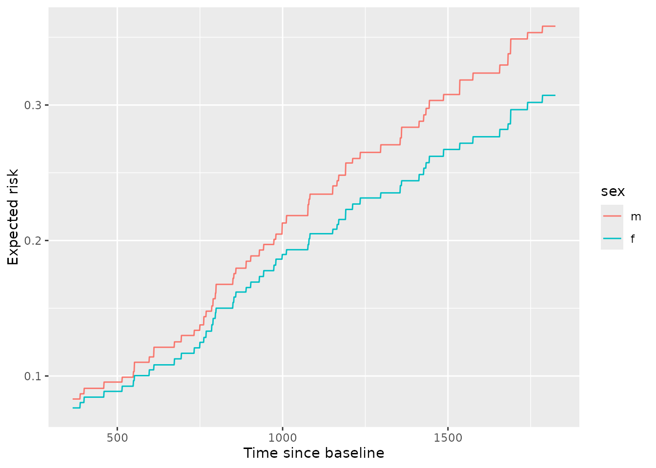
From inspection, we can see that males have higher risk than females and the difference in that risk grows over time. This can also be seen by viewing the ratio of expected risk over time:
library(data.table)

ratio_tv <- pd_sex_tv[
 , .(ratio = mean[sex == 'm'] / mean[sex == 'f']), by = pred_horizon
]

ggplot(ratio_tv, aes(x = pred_horizon, y = ratio)) +
 geom_line(color = 'grey') +
 geom_smooth(color = 'black', se = FALSE) +
 labs(x = 'time since baseline',
      y = 'ratio in expected risk for males versus females')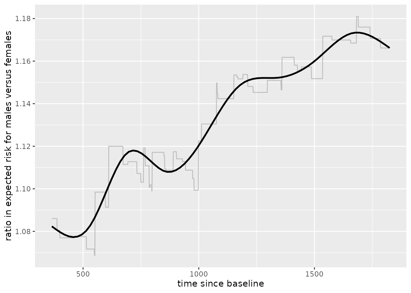
To get a view of PD for any number of variables in the training data,
use orsf_summarize_uni(). This function computes out-of-bag
PD for the most important n_variables and returns a nicely
formatted view of the output:
pd_smry <- orsf_summarize_uni(fit_surv, n_variables = 4)

pd_smry
#>
#> -- ascites (VI Rank: 1) -------------------------
#>
#>         |---------------- Risk ----------------|
#>   Value      Mean    Median     25th %    75th %
#>  <char>     <num>     <num>      <num>     <num>
#>       0 0.3083328 0.1985589 0.06581247 0.5241336
#>       1 0.4702396 0.3975953 0.27481738 0.6564321
#>
#> -- bili (VI Rank: 2) ----------------------------
#>
#>         |---------------- Risk ----------------|
#>   Value      Mean    Median     25th %    75th %
#>  <char>     <num>     <num>      <num>     <num>
#>    0.60 0.2356543 0.1536301 0.05872720 0.3719578
#>    0.80 0.2398021 0.1609720 0.06167673 0.3776136
#>    1.40 0.2613612 0.1809950 0.07893386 0.4064484
#>    3.52 0.3702763 0.3118827 0.17050712 0.5447088
#>    7.25 0.4780580 0.4406202 0.29442977 0.6434075
#>
#> -- edema (VI Rank: 3) ---------------------------
#>
#>         |---------------- Risk ----------------|
#>   Value      Mean    Median     25th %    75th %
#>  <char>     <num>     <num>      <num>     <num>
#>       0 0.3035731 0.1840849 0.06509174 0.5228237
#>     0.5 0.3558716 0.2649457 0.11132293 0.5831396
#>       1 0.4693915 0.3961470 0.28211662 0.6331870
#>
#> -- copper (VI Rank: 4) --------------------------
#>
#>         |---------------- Risk ----------------|
#>   Value      Mean    Median     25th %    75th %
#>  <char>     <num>     <num>      <num>     <num>
#>    25.5 0.2632768 0.1622871 0.05581251 0.4308234
#>    42.8 0.2707739 0.1703028 0.05887747 0.4418590
#>    74.0 0.2908707 0.1940176 0.07155433 0.4768302
#>     129 0.3444258 0.2651729 0.11918406 0.5574967
#>     214 0.4245218 0.3577346 0.21408331 0.6238041
#>
#>  Predicted risk at time t = 1826.25 for top 4 predictors
This ‘summary’ object can be converted into a data.table
for downstream plotting and tables.
head(as.data.table(pd_smry))
#>    variable importance  Value      Mean    Median     25th %    75th %
#>      <char>      <num> <char>     <num>     <num>      <num>     <num>
#> 1:  ascites  0.4960630      0 0.3083328 0.1985589 0.06581247 0.5241336
#> 2:  ascites  0.4960630      1 0.4702396 0.3975953 0.27481738 0.6564321
#> 3:     bili  0.4160074   0.60 0.2356543 0.1536301 0.05872720 0.3719578
#> 4:     bili  0.4160074   0.80 0.2398021 0.1609720 0.06167673 0.3776136
#> 5:     bili  0.4160074   1.40 0.2613612 0.1809950 0.07893386 0.4064484
#> 6:     bili  0.4160074   3.52 0.3702763 0.3118827 0.17050712 0.5447088
#>    pred_horizon  level
#>           <num> <char>
#> 1:      1826.25      0
#> 2:      1826.25      1
#> 3:      1826.25   <NA>
#> 4:      1826.25   <NA>
#> 5:      1826.25   <NA>
#> 6:      1826.25   <NA>
Multiple variables, jointly
Partial dependence can show the expected value of a model’s
predictions as a function of a specific predictor, or as a function of
multiple predictors. For instance, we can estimate predicted risk as a
joint function of bili, edema, and
trt:
pred_spec = pred_spec_auto(bili, edema, trt)

pd_bili_edema <- orsf_pd_oob(fit_surv, pred_spec)

ggplot(pd_bili_edema) +
 aes(x = bili, y = medn, col = trt, linetype = edema) +
 geom_line() +
 labs(y = 'Expected predicted risk')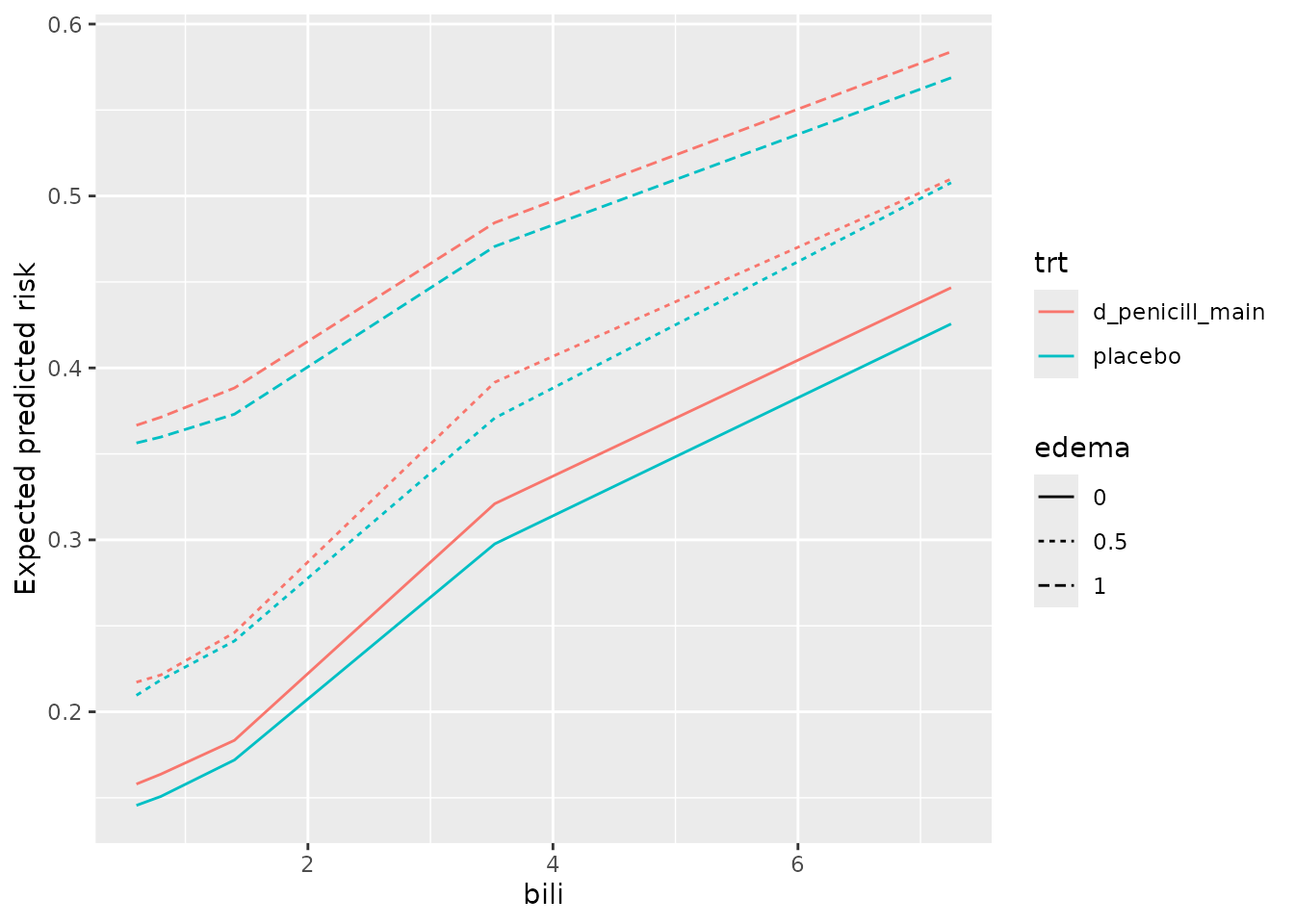
From inspection,
the model’s predictions indicate slightly lower risk for the placebo group, and these do not seem to change much at different values of
bilioredema.There is a clear increase in predicted risk with higher levels of
edemaand with higher levels ofbili-
the slope of predicted risk as a function of
biliappears highest among patients withedemaof 0.5. Is the effect ofbilimodified byedemabeing 0.5? A quick sanity check withcoxphsuggests there is.library(survival) pbc_orsf$edema_05 <- ifelse(pbc_orsf$edema == '0.5', 'yes', 'no') fit_cph <- coxph(Surv(time,status) ~ edema_05 * bili, data = pbc_orsf) anova(fit_cph) #> Analysis of Deviance Table #> Cox model: response is Surv(time, status) #> Terms added sequentially (first to last) #> #> loglik Chisq Df Pr(>|Chi|) #> NULL -550.19 #> edema_05 -546.83 6.7248 1 0.009508 ** #> bili -513.59 66.4689 1 3.555e-16 *** #> edema_05:bili -510.54 6.1112 1 0.013433 * #> --- #> Signif. codes: 0 '***' 0.001 '**' 0.01 '*' 0.05 '.' 0.1 ' ' 1
Find interactions using PD
Random forests are good at using interactions, but less good at
telling you about them. Use orsf_vint() to apply the method
for variable interaction scoring with PD described by Greenwell et al
(2018). This can take a little while if you have lots of predictors, and
it seems to work best with continuous by continuous interactions.
Interactions with categorical variables are sometimes over- or under-
scored.
# use just the continuous variables
preds <- names(fit_surv$get_means())

vint_scores <- orsf_vint(fit_surv, predictors = preds)

vint_scores
#>            interaction      score          pd_values
#>                 <char>      <num>             <list>
#>  1:   albumin..protime 1.15973071 <data.table[25x9]>
#>  2:    copper..protime 0.79587419 <data.table[25x9]>
#>  3:         bili..chol 0.74163213 <data.table[25x9]>
#>  4:          age..bili 0.74097713 <data.table[25x9]>
#>  5:       bili..copper 0.71610872 <data.table[25x9]>
#>  6:      bili..albumin 0.67849272 <data.table[25x9]>
#>  7:      bili..protime 0.59576252 <data.table[25x9]>
#>  8:       albumin..ast 0.59439149 <data.table[25x9]>
#>  9:     bili..platelet 0.56627946 <data.table[25x9]>
#> 10:       ast..protime 0.56220910 <data.table[25x9]>
#> 11:    albumin..copper 0.54057277 <data.table[25x9]>
#> 12:         bili..trig 0.52794450 <data.table[25x9]>
#> 13:       copper..trig 0.50661291 <data.table[25x9]>
#> 14:       age..protime 0.45818900 <data.table[25x9]>
#> 15:           age..ast 0.44410913 <data.table[25x9]>
#> 16:      age..platelet 0.42607794 <data.table[25x9]>
#> 17:  albumin..platelet 0.41293884 <data.table[25x9]>
#> 18:      chol..albumin 0.39547725 <data.table[25x9]>
#> 19:  platelet..protime 0.38674364 <data.table[25x9]>
#> 20:        age..copper 0.36230121 <data.table[25x9]>
#> 21:        copper..ast 0.35089611 <data.table[25x9]>
#> 22:      trig..protime 0.29339926 <data.table[25x9]>
#> 23:     bili..alk.phos 0.25729691 <data.table[25x9]>
#> 24:      chol..protime 0.24424042 <data.table[25x9]>
#> 25:   copper..alk.phos 0.22156162 <data.table[25x9]>
#> 26:          bili..ast 0.21483757 <data.table[25x9]>
#> 27:         chol..trig 0.20737852 <data.table[25x9]>
#> 28:     trig..platelet 0.18819009 <data.table[25x9]>
#> 29:      age..alk.phos 0.17844523 <data.table[25x9]>
#> 30:       chol..copper 0.17025610 <data.table[25x9]>
#> 31:   copper..platelet 0.16009542 <data.table[25x9]>
#> 32:       age..albumin 0.15186211 <data.table[25x9]>
#> 33:     alk.phos..trig 0.14212275 <data.table[25x9]>
#> 34:          age..trig 0.12185330 <data.table[25x9]>
#> 35:  albumin..alk.phos 0.12061152 <data.table[25x9]>
#> 36:          chol..ast 0.10767371 <data.table[25x9]>
#> 37:     chol..alk.phos 0.10712377 <data.table[25x9]>
#> 38:      ast..platelet 0.09157413 <data.table[25x9]>
#> 39:  alk.phos..protime 0.08277287 <data.table[25x9]>
#> 40:      alk.phos..ast 0.08062752 <data.table[25x9]>
#> 41:          ast..trig 0.07157470 <data.table[25x9]>
#> 42:          age..chol 0.05564449 <data.table[25x9]>
#> 43:     chol..platelet 0.04813670 <data.table[25x9]>
#> 44: alk.phos..platelet 0.04760897 <data.table[25x9]>
#> 45:      albumin..trig 0.04689324 <data.table[25x9]>
#>            interaction      score          pd_values
#>                 <char>      <num>             <list>
The scores include partial dependence values that you can pull out and plot:
# top scoring interaction
pd_top <- vint_scores$pd_values[[1]]

# center pd values so it's easier to see the interaction effect
pd_top[, mean := mean - mean[1], by = var_2_value]

ggplot(pd_top) +
 aes(x = var_1_value,
     y = mean,
     color = factor(var_2_value),
     group = factor(var_2_value)) +
 geom_line() +
 labs(x = "albumin",
      y = "predicted mortality (centered)",
      color = "protime")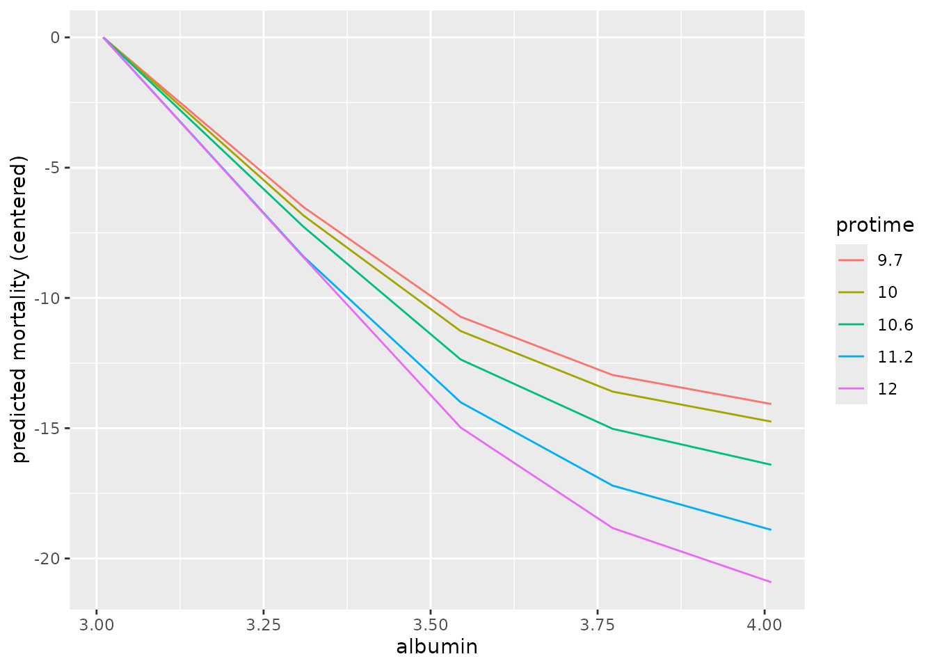
Again we use a sanity check with coxph to see if these
interactions are detected using a standard test:
# test the top score (expect strong interaction)
fit_cph <- coxph(Surv(time,status) ~ albumin * protime,
                 data = pbc_orsf)

anova(fit_cph)
#> Analysis of Deviance Table
#>  Cox model: response is Surv(time, status)
#> Terms added sequentially (first to last)
#>
#>                  loglik  Chisq Df Pr(>|Chi|)
#> NULL            -550.19
#> albumin         -526.29 47.801  1  4.717e-12 ***
#> protime         -514.89 22.806  1  1.792e-06 ***
#> albumin:protime -511.76  6.252  1    0.01241 *
#> ---
#> Signif. codes: 0 '***' 0.001 '**' 0.01 '*' 0.05 '.' 0.1 ' ' 1Note: Caution is warranted when interpreting statistical hypotheses that are motivated by the same data they are tested with. Results like the p-values for interaction shown above should be interpreted as exploratory.
Individual conditional expectations (ICE)
Unlike partial dependence, which shows the expected prediction as a function of one or multiple predictors, individual conditional expectations (ICE) show the prediction for an individual observation as a function of a predictor.
Classification
Compute ICE using out-of-bag data for
flipper_length_mm = c(190, 210).
pred_spec <- list(flipper_length_mm = c(190, 210))

ice_oob <- orsf_ice_oob(fit_clsf, pred_spec = pred_spec)

ice_oob
#> Key: <class>
#>      id_variable id_row  class flipper_length_mm       pred
#>            <int> <char> <fctr>             <num>      <num>
#>   1:           1      1 Adelie               190 0.92045213
#>   2:           1      2 Adelie               190 0.80427932
#>   3:           1      3 Adelie               190 0.84342550
#>   4:           1      4 Adelie               190 0.93514694
#>   5:           1      5 Adelie               190 0.97172229
#>  ---
#> 896:           2    146 Gentoo               210 0.25779089
#> 897:           2    147 Gentoo               210 0.04806888
#> 898:           2    148 Gentoo               210 0.07926342
#> 899:           2    149 Gentoo               210 0.84597108
#> 900:           2    150 Gentoo               210 0.10191162
There are two identifiers in the output:
id_variableis an identifier for the current value of the variable(s) that are in the data. It is redundant if you only have one variable, but helpful if there are multiple variables.id_rowis an identifier for the observation in the original data.
Note that predicted probabilities are returned for each class and each observation in the data. Predicted probabilities for a given observation and given variable value sum to 1. For example,
#> [1] 1Regression
Compute ICE using new data for
flipper_length_mm = c(190, 210).
pred_spec <- list(flipper_length_mm = c(190, 210))

ice_new <- orsf_ice_new(fit_regr,
                        pred_spec = pred_spec,
                        new_data = penguins_orsf_test)

ice_new
#>      id_variable id_row flipper_length_mm     pred
#>            <int> <char>             <num>    <num>
#>   1:           1      1               190 37.94483
#>   2:           1      2               190 37.61595
#>   3:           1      3               190 37.53681
#>   4:           1      4               190 39.49476
#>   5:           1      5               190 38.95635
#>  ---
#> 362:           2    179               210 51.80471
#> 363:           2    180               210 47.27183
#> 364:           2    181               210 47.05031
#> 365:           2    182               210 50.39028
#> 366:           2    183               210 48.44774
You can also let pred_spec_auto pick reasonable values
like so:
pred_spec = pred_spec_auto(species, island, body_mass_g)

ice_new <- orsf_ice_new(fit_regr,
                        pred_spec = pred_spec,
                        new_data = penguins_orsf_test)

ice_new
#>       id_variable id_row species    island body_mass_g     pred
#>             <int> <char>  <fctr>    <fctr>       <num>    <num>
#>    1:           1      1  Adelie    Biscoe        3200 37.78339
#>    2:           1      2  Adelie    Biscoe        3200 37.73273
#>    3:           1      3  Adelie    Biscoe        3200 37.71248
#>    4:           1      4  Adelie    Biscoe        3200 40.25782
#>    5:           1      5  Adelie    Biscoe        3200 40.04074
#>   ---
#> 8231:          45    179  Gentoo Torgersen        5300 46.14559
#> 8232:          45    180  Gentoo Torgersen        5300 43.98050
#> 8233:          45    181  Gentoo Torgersen        5300 44.59837
#> 8234:          45    182  Gentoo Torgersen        5300 44.85146
#> 8235:          45    183  Gentoo Torgersen        5300 44.23710
By default, all combinations of all variables are used. However, you can also look at the variables one by one, separately, like so:
ice_new <- orsf_ice_new(fit_regr,
                        expand_grid = FALSE,
                        pred_spec = pred_spec,
                        new_data = penguins_orsf_test)

ice_new
#>       id_variable id_row    variable value  level     pred
#>             <int> <char>      <char> <num> <char>    <num>
#>    1:           1      1     species    NA Adelie 37.74136
#>    2:           1      2     species    NA Adelie 37.42367
#>    3:           1      3     species    NA Adelie 37.04598
#>    4:           1      4     species    NA Adelie 39.89602
#>    5:           1      5     species    NA Adelie 39.14848
#>   ---
#> 2009:           5    179 body_mass_g  5300   <NA> 51.50196
#> 2010:           5    180 body_mass_g  5300   <NA> 47.27055
#> 2011:           5    181 body_mass_g  5300   <NA> 48.34064
#> 2012:           5    182 body_mass_g  5300   <NA> 48.75828
#> 2013:           5    183 body_mass_g  5300   <NA> 48.11020
And you can also bypass all the bells and whistles by using your own
data.frame for a pred_spec. (Just make sure
you request values that exist in the training data.)
custom_pred_spec <- data.frame(species = 'Adelie',
                               island = 'Biscoe')

ice_new <- orsf_ice_new(fit_regr,
                        pred_spec = custom_pred_spec,
                        new_data = penguins_orsf_test)

ice_new
#>      id_variable id_row species island     pred
#>            <int> <char>  <fctr> <fctr>    <num>
#>   1:           1      1  Adelie Biscoe 38.52327
#>   2:           1      2  Adelie Biscoe 38.32073
#>   3:           1      3  Adelie Biscoe 37.71248
#>   4:           1      4  Adelie Biscoe 41.68380
#>   5:           1      5  Adelie Biscoe 40.91140
#>  ---
#> 179:           1    179  Adelie Biscoe 43.09493
#> 180:           1    180  Adelie Biscoe 38.79455
#> 181:           1    181  Adelie Biscoe 39.37734
#> 182:           1    182  Adelie Biscoe 40.71952
#> 183:           1    183  Adelie Biscoe 39.34501
Survival
Compute ICE using in-bag data for
bili = c(1,2,3,4,5):
ice_train <- orsf_ice_inb(fit_surv, pred_spec = list(bili = 1:5))
ice_train
#>       id_variable id_row pred_horizon  bili      pred
#>             <int> <char>        <num> <num>     <num>
#>    1:           1      1      1826.25     1 0.9015162
#>    2:           1      2      1826.25     1 0.1019426
#>    3:           1      3      1826.25     1 0.6821646
#>    4:           1      4      1826.25     1 0.3623411
#>    5:           1      5      1826.25     1 0.1374271
#>   ---
#> 1376:           5    272      1826.25     5 0.2650957
#> 1377:           5    273      1826.25     5 0.3065318
#> 1378:           5    274      1826.25     5 0.3503776
#> 1379:           5    275      1826.25     5 0.1652897
#> 1380:           5    276      1826.25     5 0.3549165
If you don’t have specific values of a variable in mind, let
pred_spec_auto pick for you:
ice_train <- orsf_ice_inb(fit_surv, pred_spec_auto(bili))
ice_train
#>       id_variable id_row pred_horizon  bili       pred
#>             <int> <char>        <num> <num>      <num>
#>    1:           1      1      1826.25  0.60 0.89210440
#>    2:           1      2      1826.25  0.60 0.09186876
#>    3:           1      3      1826.25  0.60 0.65503431
#>    4:           1      4      1826.25  0.60 0.34622748
#>    5:           1      5      1826.25  0.60 0.13310425
#>   ---
#> 1376:           5    272      1826.25  7.25 0.31258148
#> 1377:           5    273      1826.25  7.25 0.35478676
#> 1378:           5    274      1826.25  7.25 0.41559176
#> 1379:           5    275      1826.25  7.25 0.25301890
#> 1380:           5    276      1826.25  7.25 0.44533769
Specify pred_horizon to get ICE at each value:
ice_train <- orsf_ice_inb(fit_surv, pred_spec_auto(bili),
                          pred_horizon = seq(500, 3000, by = 500))
ice_train
#>       id_variable id_row pred_horizon  bili      pred
#>             <int> <char>        <num> <num>     <num>
#>    1:           1      1          500  0.60 0.5949598
#>    2:           1      1         1000  0.60 0.7652137
#>    3:           1      1         1500  0.60 0.8751746
#>    4:           1      1         2000  0.60 0.9057135
#>    5:           1      1         2500  0.60 0.9231915
#>   ---
#> 8276:           5    276         1000  7.25 0.2111306
#> 8277:           5    276         1500  7.25 0.3642278
#> 8278:           5    276         2000  7.25 0.4850492
#> 8279:           5    276         2500  7.25 0.5720362
#> 8280:           5    276         3000  7.25 0.6206786
Multi-prediction horizon ice comes with minimal extra computational cost. Use a fine grid of time values and assess whether predictors have time-varying effects.
Visualizing ICE curves
Inspecting the ICE curves for each observation can help identify whether there is heterogeneity in a model’s predictions. I.e., does the effect of the variable follow the same pattern for all the data, or are there groups where the variable impacts risk differently?
I am going to turn off boundary checking in orsf_ice_oob
by setting boundary_checks = FALSE, and this will allow me
to generate ICE curves that go beyond the 90th percentile of
bili.
pred_spec <- list(bili = seq(1, 10, length.out = 25))

ice_oob <- orsf_ice_oob(fit_surv, pred_spec, boundary_checks = FALSE)

ice_oob
#>       id_variable id_row pred_horizon  bili      pred
#>             <int> <char>        <num> <num>     <num>
#>    1:           1      1      1826.25     1 0.8790861
#>    2:           1      2      1826.25     1 0.8132035
#>    3:           1      3      1826.25     1 0.6240238
#>    4:           1      4      1826.25     1 0.7461603
#>    5:           1      5      1826.25     1 0.5754091
#>   ---
#> 6896:          25    272      1826.25    10 0.7018976
#> 6897:          25    273      1826.25    10 0.4606246
#> 6898:          25    274      1826.25    10 0.3347082
#> 6899:          25    275      1826.25    10 0.6046024
#> 6900:          25    276      1826.25    10 0.2789017
For plots, it is helpful to scale the ICE data. I subtract the
initial value of predicted risk (i.e., when bili = 1) from
each observation’s conditional expectation values. So,
Every curve start at 0
-
The plot shows change in predicted risk as a function of
bili.ice_oob[, pred_subtract := rep(pred[id_variable==1], times=25)] ice_oob[, pred := pred - pred_subtract]
Now we can visualize the curves.
ggplot(ice_oob, aes(x = bili,
                    y = pred,
                    group = id_row)) +
 geom_line(alpha = 0.15) +
 labs(y = 'Change in predicted risk') +
 geom_smooth(se = FALSE, aes(group = 1))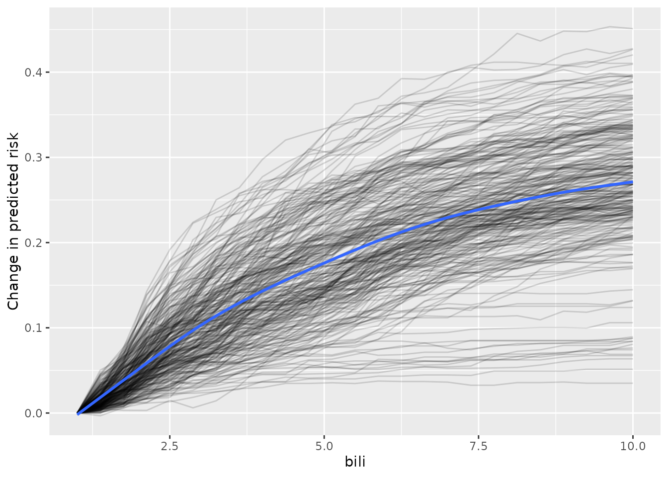
From inspection of the figure,
Most of the individual slopes cluster around the overall trend - Good!
A small number of individual slopes appear to be flat. It may be helpful to investigate this further.
Limitations of PD
Partial dependence has a number of known limitations and assumptions that users should be aware of (see Hooker, 2021). In particular, partial dependence is less intuitive when >2 predictors are examined jointly, and it is assumed that the feature(s) for which the partial dependence is computed are not correlated with other features (this is likely not true in many cases). Accumulated local effect plots can be used (see here) in the case where feature independence is not a valid assumption.