library(birdsize)
library(dplyr)
#>
#> Attaching package: 'dplyr'
#> The following objects are masked from 'package:stats':
#>
#>     filter, lag
#> The following objects are masked from 'package:base':
#>
#>     intersect, setdiff, setequal, union
library(ggplot2)
theme_set(theme_bw())
Overview
birdsize simulates mass measurements (in g) for birds.
Working from the assumption that individuals of a species have body
masses normally distributed around a species-wide mean and standard
deviation, birdsize simulates individual-level body mass
measurements by drawing from species-specific normal distributions.
There are parameters built-in for 450 bird species, or a user may supply
mean and optionally standard deviation values for additional
species.
The core functions in birdsize apply at 3 levels of
organization: species, population, and community:
- The
species_*functions take information about a real or hypothetical species and look up or calculate the parameters necessary to simulate body size distributions for that species. - The
population_*functions use species-level parameters and abundances (population sizes) to simulate individual body size and basal metabolic rate measurements to make up populations of that species. - The
community_*functions generate individual body mass estimates for multiple populations in one go (e.g. populations of different species, or populations of the same species at different points in time or different sampling locations).
Species-level parameters
In order to generate body mass estimates for a species,
birdsize needs an abundance value (how many
individuals to generate estimates for) and at least one of:
- For one of the 450 species known to
birdsize: the scientific name (as"Genus species") or the AOU numeric code. See LINK for a list of the species with data included inbirdsize. - For any other species: the mean body mass (in g) for that species. If a standard deviation value is provided, it will be used. Otherwise, it will be estimated based on the mean body mass via the scaling relationship described in the scaling vignette.
The species_define function uses the information
provided to look up, or calculate, the mean and standard deviation of
body mass to use to generate individuals of the desired species. This
function usually operates under the hood, but may be of interest to
advanced users or those interested in complex simulations involving
changes to the species-wide parameters.
Population (one species) simulations
Using species identity
For the birds known to birdsize you can use the species’
code (AOU) to simulate a population directly. For the hummingbird
Selasphorus calliope:
a_hundred_hummingbirds <- pop_generate(abundance = 100, AOU = 4360)

head(a_hundred_hummingbirds)
#>    AOU sim_species_id individual_mass individual_bmr mean_size   sd_size
#> 1 4360           4360        2.556873       20.50623      2.65 0.1818394
#> 2 4360           4360        3.101904       23.53533      2.65 0.1818394
#> 3 4360           4360        2.833263       22.06327      2.65 0.1818394
#> 4 4360           4360        2.703245       21.33652      2.65 0.1818394
#> 5 4360           4360        2.612003       20.82052      2.65 0.1818394
#> 6 4360           4360        2.987874       22.91515      2.65 0.1818394
#>   abundance  sd_method      scientific_name
#> 1       100 AOU lookup Selasphorus calliope
#> 2       100 AOU lookup Selasphorus calliope
#> 3       100 AOU lookup Selasphorus calliope
#> 4       100 AOU lookup Selasphorus calliope
#> 5       100 AOU lookup Selasphorus calliope
#> 6       100 AOU lookup Selasphorus calliope

ggplot(a_hundred_hummingbirds, aes(individual_mass)) +
  geom_histogram(bins = 25) +
  xlab("Mass (g)") +
  ylab("Count") +
  ggtitle("A population of hummingbirds")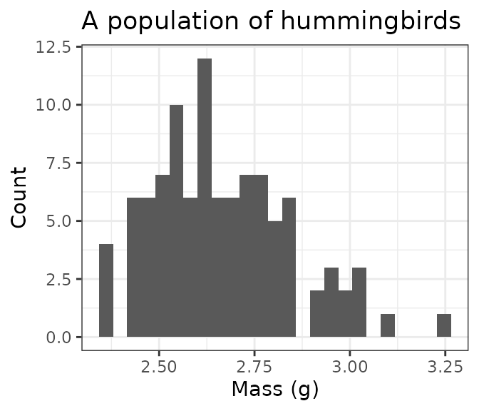
Using a known mean and standard deviation
Alternatively, you can simulate body masses for a population by
supplying the body size parameters yourself. This may be useful if you
would like to work with a species not included in birdsize,
test sensitivities to different parameter ranges, or generate values for
simulation/null models (or, other applications!).
Note that, if both mean mass and a species code are provided, the species code will be used and the mean mass provided will be ignored!
a_hundred_hypotheticals <- pop_generate(abundance = 100, mean_size = 25, sd_size = 3)

head(a_hundred_hypotheticals)
#>   AOU sim_species_id individual_mass individual_bmr mean_size sd_size abundance
#> 1  NA              1        19.86281       88.44888        25       3       100
#> 2  NA              1        22.60234       96.98414        25       3       100
#> 3  NA              1        20.76744       91.30263        25       3       100
#> 4  NA              1        26.59827      108.92055        25       3       100
#> 5  NA              1        23.80690      100.64180        25       3       100
#> 6  NA              1        24.14694      101.66465        25       3       100
#>              sd_method scientific_name
#> 1 Mean and SD provided            <NA>
#> 2 Mean and SD provided            <NA>
#> 3 Mean and SD provided            <NA>
#> 4 Mean and SD provided            <NA>
#> 5 Mean and SD provided            <NA>
#> 6 Mean and SD provided            <NA>

ggplot(a_hundred_hypotheticals, aes(individual_mass)) +
  geom_histogram(bins = 25) +
  xlab("Mass (g)") +
  ylab("Count") +
  ggtitle("A population of hypothetical birds", subtitle = "Mean mass = 25 g\nStandard deviation = 3")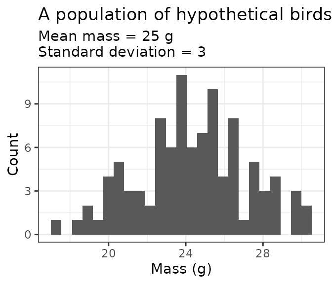
Using a known mean, but no standard deviation
If the mean mass is not known or not provided,
pop_generate will estimate the standard deviation based on
scaling between the mean and standard deviation of body mass:
another_hundred_hypotheticals <- pop_generate(abundance = 100, mean_size = 25)

head(another_hundred_hypotheticals)
#>   AOU sim_species_id individual_mass individual_bmr mean_size  sd_size
#> 1  NA              1        26.24416      107.88463        25 1.746196
#> 2  NA              1        21.44791       93.42580        25 1.746196
#> 3  NA              1        20.79538       91.39020        25 1.746196
#> 4  NA              1        23.75958      100.49914        25 1.746196
#> 5  NA              1        22.17191       95.66364        25 1.746196
#> 6  NA              1        22.58620       96.93474        25 1.746196
#>   abundance              sd_method scientific_name
#> 1       100 SD estimated from mean            <NA>
#> 2       100 SD estimated from mean            <NA>
#> 3       100 SD estimated from mean            <NA>
#> 4       100 SD estimated from mean            <NA>
#> 5       100 SD estimated from mean            <NA>
#> 6       100 SD estimated from mean            <NA>

ggplot(another_hundred_hypotheticals, aes(individual_mass)) +
  geom_histogram(bins = 25) +
  xlab("Mass (g)") +
  ylab("Count") +
  ggtitle("A population of hypothetical birds", subtitle = "Mean mass = 25 g\nStandard deviation = 1.74")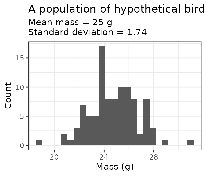
Community (multiple populations) simulations
community_generate takes a dataframe with species-level
information (AOU, scientific name, or mean and/or standard deviation
body mass) and population sizes, and returns a dataframe of
individual-level mass and BMR measurements for all the entries in the
input data frame.
Simulations using AOU
Here, we use a synthetic dataset with records of AOU and
abundance for 5 species, to make up a community:
data("toy_aou_community")

head(toy_aou_community)
#> # A tibble: 5 × 2
#>     AOU abundance
#>   <dbl>     <dbl>
#> 1  4730        95
#> 2  3000        40
#> 3  3280        63
#> 4  3860        69
#> 5  4460        53
community_generate can take this table and generate
simulated individual measurements with no additional tweaks. It uses the
AOU and abundance columns from
toy_aou_community to look up species’ mean and standard
deviation body masses based on their AOU and then draw individual size
measurements from a normal distribution with those parameters.
toy_aou_sims <- community_generate(community_data_table = toy_aou_community, abundance_column_name = "abundance")

head(toy_aou_sims)
#>    AOU sim_species_id individual_mass individual_bmr mean_size  sd_size
#> 1 4730           4730        38.82847       142.6440    37.475 3.300613
#> 2 4730           4730        40.41270       146.7697    37.475 3.300613
#> 3 4730           4730        42.74367       152.7569    37.475 3.300613
#> 4 4730           4730        34.45230       130.9863    37.475 3.300613
#> 5 4730           4730        36.21842       135.7394    37.475 3.300613
#> 6 4730           4730        42.32158       151.6799    37.475 3.300613
#>   abundance  sd_method scientific_name
#> 1        95 AOU lookup Alauda arvensis
#> 2        95 AOU lookup Alauda arvensis
#> 3        95 AOU lookup Alauda arvensis
#> 4        95 AOU lookup Alauda arvensis
#> 5        95 AOU lookup Alauda arvensis
#> 6        95 AOU lookup Alauda arvensis
The resulting table has one row per individual, with a unique
individual_size and individual_bmr estimate
for that individual.
We can then plot the individual size distribution for the community, colored by species ID:
toy_aou_sims$`Scientific name` = toy_aou_sims$scientific_name

ggplot(toy_aou_sims, aes(individual_mass, fill = `Scientific name`)) +
  geom_histogram(position = "stack") +
  scale_fill_viridis_d() +
  scale_x_log10() +
  ggtitle("Community simulated via AOU") +
  xlab("Body mass (g)") +
  ylab("Number of individuals") +
  theme(legend.position = "bottom", legend.direction = "vertical")
#> `stat_bin()` using `bins = 30`. Pick better value `binwidth`.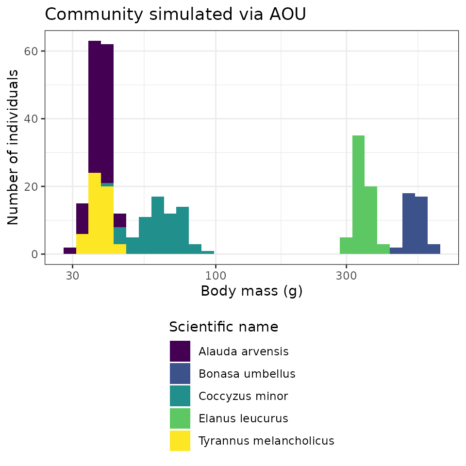
Simulation given species’ names
If the AOU is not known or not provided,
community_generate will attempt to look up species’ size
parameters based on their scientific name.
data("toy_species_name_community")

head(toy_species_name_community)
#> # A tibble: 5 × 2
#>   scientific_name        abundance
#>   <chr>                      <dbl>
#> 1 Alauda arvensis               95
#> 2 Bonasa umbellus               40
#> 3 Elanus leucurus               63
#> 4 Coccyzus minor                69
#> 5 Tyrannus melancholicus        53
community_generate still runs, but note that the
sd_method here is listed as
Scientific name lookup rather than AOU lookup
(above).
toy_species_name_sims <- community_generate(toy_species_name_community, abundance_column_name = "abundance")

head(toy_species_name_sims)
#>    AOU sim_species_id individual_mass individual_bmr mean_size  sd_size
#> 1 4730           4730        39.97640       145.6382    37.475 3.300613
#> 2 4730           4730        38.37580       141.4563    37.475 3.300613
#> 3 4730           4730        37.62253       139.4709    37.475 3.300613
#> 4 4730           4730        39.98764       145.6674    37.475 3.300613
#> 5 4730           4730        38.66003       142.2025    37.475 3.300613
#> 6 4730           4730        37.95838       140.3575    37.475 3.300613
#>   abundance              sd_method scientific_name
#> 1        95 Scientific name lookup Alauda arvensis
#> 2        95 Scientific name lookup Alauda arvensis
#> 3        95 Scientific name lookup Alauda arvensis
#> 4        95 Scientific name lookup Alauda arvensis
#> 5        95 Scientific name lookup Alauda arvensis
#> 6        95 Scientific name lookup Alauda arvensis
toy_species_name_sims$`Scientific name` = toy_species_name_sims$scientific_name

ggplot(toy_species_name_sims, aes(individual_mass, fill = scientific_name)) +
  geom_histogram(position = "stack") +
  scale_fill_viridis_d() +
  scale_x_log10() +
  ggtitle("Community simulated via scientific name") +
  xlab("Body mass (g)") +
  ylab("Number of individuals") +
  theme(legend.position = "bottom", legend.direction = "vertical")
#> `stat_bin()` using `bins = 30`. Pick better value `binwidth`.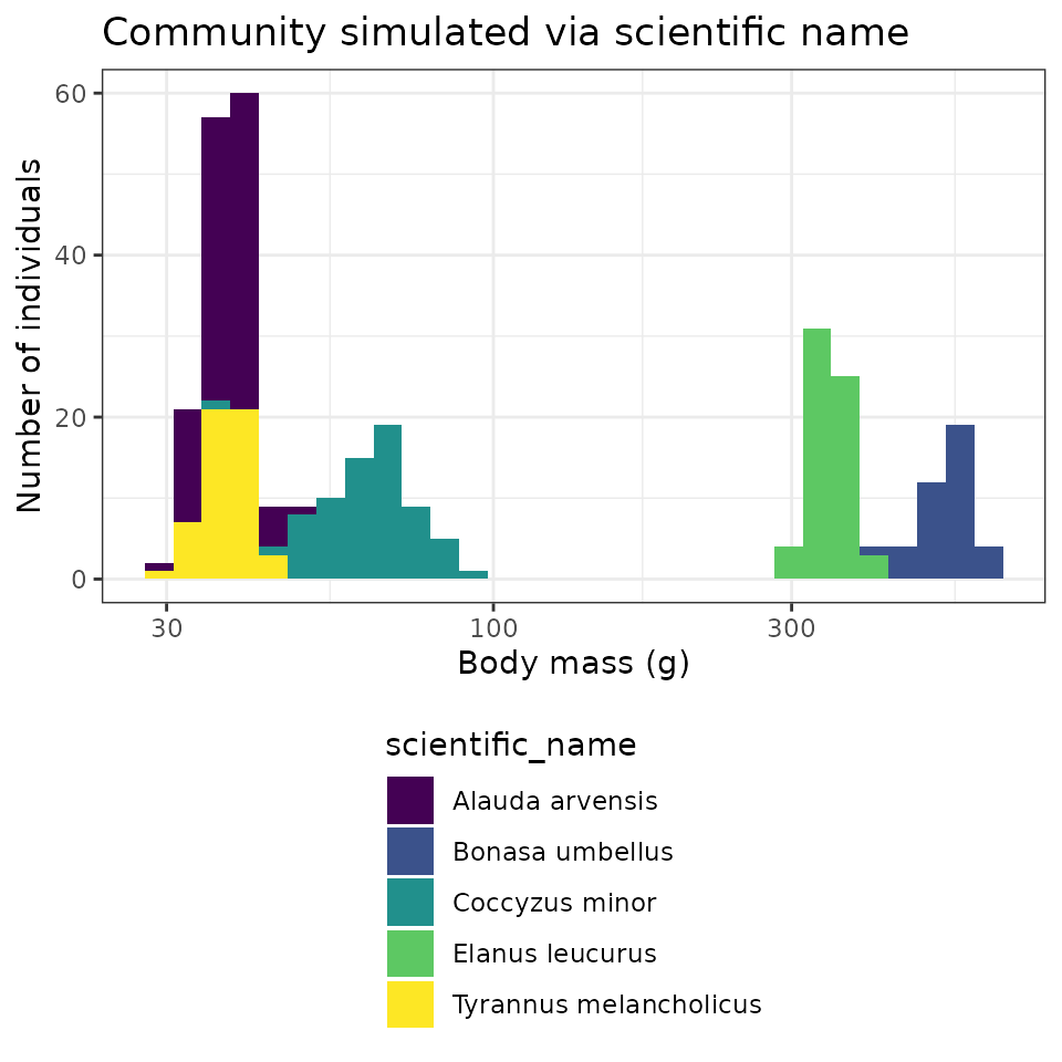
Simulation given mean size measurements
If species name or AOU are not known, or are not included in this
dataset (see known_species for the full set of included
species), estimates can still be generated by providing the mean and, if
available, standard deviation of body mass directly. If standard
deviation is provided, it will be used; if not, it will be estimated
based on the scaling relationship between mean and standard deviation of
body mass for birds (see the scaling vignette).
This functionality may be especially useful for users interested in
using their own parameter values, rather than relying on the ones
provided in birdsize. For example, birdsize
does not take into account temporal or geographic variation in body
size, which may be significant. A user could manually provide values to
explore these scenarios.
Note that 1) the mean body size data must be provided in a column
named mean_size and 2) the sim_species_id
column acts as a species identifier in the absence of other taxonomic
information:
data(toy_size_community)

head(toy_size_community)
#> # A tibble: 5 × 3
#>   abundance mean_size sim_species_id
#>       <dbl>     <dbl>          <int>
#> 1        95      37.5              1
#> 2        40     532                2
#> 3        63     346                3
#> 4        69      63.9              4
#> 5        53      37.4              5
toy_size_sims <- community_generate(toy_size_community, abundance_column_name = "abundance")

head(toy_size_sims)
#>   AOU sim_species_id individual_mass individual_bmr mean_size  sd_size
#> 1  NA              1        39.74559       145.0382    37.475 2.625949
#> 2  NA              1        38.47302       141.7117    37.475 2.625949
#> 3  NA              1        35.73167       134.4362    37.475 2.625949
#> 4  NA              1        41.46384       149.4816    37.475 2.625949
#> 5  NA              1        38.36155       141.4188    37.475 2.625949
#> 6  NA              1        37.59558       139.3997    37.475 2.625949
#>   abundance              sd_method scientific_name
#> 1        95 SD estimated from mean            <NA>
#> 2        95 SD estimated from mean            <NA>
#> 3        95 SD estimated from mean            <NA>
#> 4        95 SD estimated from mean            <NA>
#> 5        95 SD estimated from mean            <NA>
#> 6        95 SD estimated from mean            <NA>
toy_size_sims$`Sim species ID` <- as.character(toy_size_sims$sim_species_id)

ggplot(toy_size_sims, aes(individual_mass, fill = `Sim species ID`)) +
  geom_histogram(position = "stack") +
  scale_fill_viridis_d() +
  scale_x_log10() +
  ggtitle("Community simulated via mean body size") +
  xlab("Body mass (g)") +
  ylab("Number of individuals") +
  theme(legend.position = "bottom")
#> `stat_bin()` using `bins = 30`. Pick better value `binwidth`.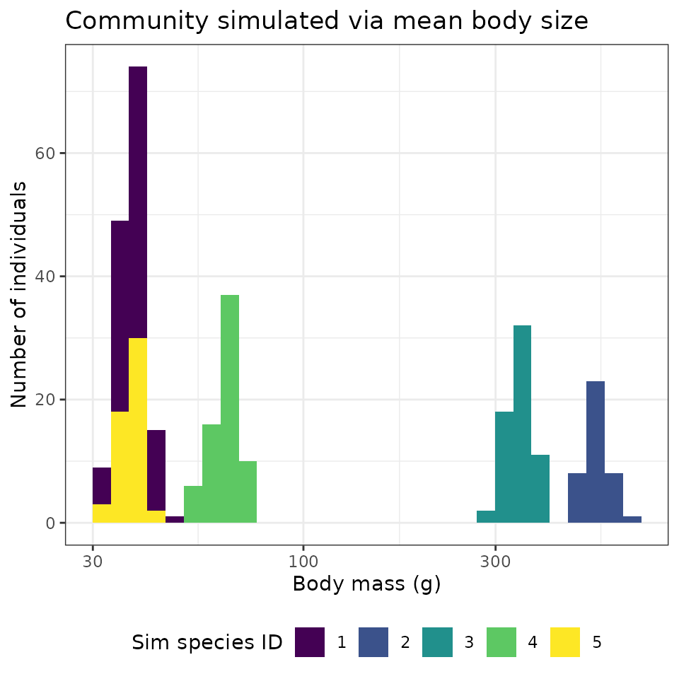
Community-wide summary statistics
The body size measurements generated by birdsize are
estimates and are generally best-suited for large-scale, aggregate
analyses. For these bigger-picture analyses, use general aggregation and
summary functions to generate community-wide summaries.
For example, using dplyr:
Biomass total by species
toy_species_name_sims_summary <-
  toy_species_name_sims |>
  group_by(scientific_name) |>
  summarize(
    total_mass = sum(individual_mass),
    total_n_individuals = n()
  )

toy_species_name_sims_summary
#> # A tibble: 5 × 3
#>   scientific_name        total_mass total_n_individuals
#>   <chr>                       <dbl>               <int>
#> 1 Alauda arvensis             3566.                  95
#> 2 Bonasa umbellus            21273.                  40
#> 3 Coccyzus minor              4409.                  69
#> 4 Elanus leucurus            21765.                  63
#> 5 Tyrannus melancholicus      1980.                  53