Introduction to chirps
Kauê de Sousa
Department of Agricultural Sciences, University of Inland Norway, Hamar, Norway Digital Inclusion, Bioversity International, Montpellier, FranceAdam H. Sparks
Centre for Crop Health, University of Southern Queensland, Toowoomba, AustraliaAniruddha Ghosh
Climate Action, International Center for Tropical Agriculture (CIAT), Nairobi, KenyaSource:
vignettes/Overview.Rmd
Overview.RmdSummary
The chirps package (de Sousa et al. 2020) provides
functionalities for reproducible analysis using the CHIRPS (Funk et al. 2015) and CHIRTS data (Funk et al. 2019). CHIRPS is a daily
precipitation data set developed by the Climate Hazards Group for high
resolution precipitation gridded data. Spanning 50°S - 50°N (and all
longitudes) and ranging from 1981 to near-present (normally with a 45
day lag), CHIRPS incorporates 0.05 arc-degree resolution satellite
imagery, and in-situ station data to create gridded precipitation time
series for trend analysis and seasonal drought monitoring. CHIRTS is a
quasi-global (60°S – 70°N), high-resolution data set of daily maximum
and minimum temperatures.
Other functionalities of chirps are the computation of
precipitation indices, the retrieval of the evaporative stress index
(ESI) which describes temporal anomalies in evapotranspiration produced
weekly at 0.25 arc-degree resolution for the entire globe, and the
retrieval of IMERG data which provides near-real time global
observations of rainfall at 0.5 arc-degree resolution.
CHIRPS (precipitation data)
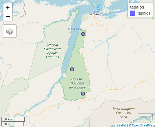
The Tapajós National Forest is a protected area in the
Brazilian Amazon. Located within the coordinates -55.4° and -54.8°E and
-4.1° and -2.7°S with ~527,400 ha of multiple Amazonian ecosystems. We
take three points within its area to get the precipitation from Jan-2013
to Dec-2018 using get_chirps().

For this example we fetch the data from the server “ClimateSERV”
using the argument server = "ClimateSERV". This option is
recommended when working with few data points as the request could be
faster. The default server = "CHC" is used for multiple
data points and years.
library("chirps")
library("sf")

data("tapajos", package = "chirps")

# sample three points within the Tapajos area
set.seed(1234)
tp_point = st_sample(tapajos, 3)

# coerce as sf points
tp_point = st_as_sf(tp_point)

dat = get_chirps(tp_point,
                 dates = c("2013-01-01","2018-12-31"),
                 server = "ClimateSERV")
#> Fetching data from ClimateSERV
#> Getting your request...
Precipitation indices
By default, the function get_chirps() returns a
data.frame which inherits the classes ‘chirps’ and ‘chirps_df’, where
each id represents the index for the rows in the in-putted ‘object’. It
is possible to return the data as a matrix using the argument
as.matrix = TRUE.
dat
#>          id    lon   lat       date chirps
#>       <int>  <dbl> <dbl>     <date>  <dbl>
#> 1:        1 -55.03 -3.80 2013-01-01   0.00
#> 2:        1 -55.03 -3.80 2013-01-02  12.36
#> 3:        1 -55.03 -3.80 2013-01-03  24.72
#> 4:        1 -55.03 -3.80 2013-01-04   0.00
#> 5:        1 -55.03 -3.80 2013-01-05   0.00
#> ---
#> 6569:     3 -55.03 -3.41 2018-12-27   0.00
#> 6570:     3 -55.03 -3.41 2018-12-28   0.00
#> 6571:     3 -55.03 -3.41 2018-12-29   0.00
#> 6572:     3 -55.03 -3.41 2018-12-30   0.00
#> 6573:     3 -55.03 -3.41 2018-12-31   0.00
With precip_indices() is possible to assess how the
precipitation changes across a time series using precipitation
variability indices (Aguilar et al. 2005).
Here, we take the indices for intervals of 15 days and compute the
indices for the time series (from Jan-2013 to Dec-2018).
p_ind = precip_indices(dat, timeseries = TRUE, intervals = 15)

p_ind
#>          id       date    lon   lat  index  value
#>       <int>     <date>  <dbl> <dbl>  <chr>  <dbl>
#> 1:        1 2013-01-01 -55.03 -3.80   MLDS   7.00
#> 2:        1 2013-01-01 -55.03 -3.80   MLWS   2.00
#> 3:        1 2013-01-01 -55.03 -3.80  R10mm   1.00
#> 4:        1 2013-01-01 -55.03 -3.80  R20mm   3.00
#> 5:        1 2013-01-01 -55.03 -3.80 Rx1day  45.70
#> ---
#> 3446:     3 2018-12-16 -55.03 -3.41 Rx5day  53.90
#> 3447:     3 2018-12-16 -55.03 -3.41   R95p  34.53
#> 3448:     3 2018-12-16 -55.03 -3.41   R99p  34.53
#> 3449:     3 2018-12-16 -55.03 -3.41 Rtotal  80.49
#> 3450:     3 2018-12-16 -55.03 -3.41   SDII  13.42
The function precip_indices() returns a data.frame with
the precipitation indices. Each date corresponds to the first day in the
time series intervals as defined by the argument ‘intervals’. When
timeseries = FALSE the function returns a single
precipitation index for the entire time series.
CHIRTS (temperature data)
Maximum and minimum temperature and relative humidity data are
available with the function get_chirts(). Data is requested
to the server CHC as default and is currently available from 1983 to
2016. We use the same random points from the Tapajós National Forest but
for few days to speed up the call.
dates = c("2010-12-15","2010-12-31")

temp1 = get_chirts(tp_point, dates, var = "Tmax", as.matrix = TRUE)

temp2 = get_chirts(tp_point, dates, var = "Tmin", as.matrix = TRUE)

rhu = get_chirts(tp_point, dates, var = "RHum", as.matrix = TRUE)
Going further
Evapotranspiration
The chirps package also retrieves the Evaporative Stress
Index (ESI) using the function get_esi() which behaves
similarly as get_chirps().
The function get_esi() may return NAs due
to cloudiness in the dataset. Which will return an error message:
set.seed(123)
lonlat = data.frame(lon = runif(1, -55, -54),
                    lat = runif(1, -3, -2.7))

get_esi(lonlat, c("2017-12-01","2018-01-20"))
One way to deal with this is increase the buffer area around the
in-putted object with the argument dist passed to
st_buffer() from sf (Pebesma 2018) through the ...
functionality in get_esi(). The argument
nQuadSegs defines the number of segments per quadrant in
the buffer.
Objects of class sf
To return an object with the same class (sf), the
argument as.sf = TRUE is used.
get_chirps(tapajos, dates = c("2017-12-15","2017-12-31"), as.sf = TRUE)Objects of class geojson
get_chirps() and get_esi() also contains a
method for objects of class geojson with geometries ‘Point’ and
‘Polygon’. To return an object with the same class
(geojson), the argument as.geojson = TRUE is
used.