Introduction
-
chopinautomatically distributes geospatial data computation over multiple threads. - Function centered workflow will streamline the process of parallelizing geospatial computation with minimal effort.
chopin workflow
- The simplest way of parallelizing generic geospatial computation is
to start from
par_pad_*functions topar_grid, or runningpar_hierarchy, orpar_multirastersfunctions at once.
Example data
- North Carolinian counties and a raster of elevation data are used as example data.
temp_dir <- tempdir(check = TRUE)

url_nccnty <-
  paste0(
    "https://raw.githubusercontent.com/",
    "ropensci/chopin/refs/heads/main/",
    "tests/testdata/nc_hierarchy.gpkg"
  )
url_ncelev <-
  paste0(
    "https://raw.githubusercontent.com/",
    "ropensci/chopin/refs/heads/main/",
    "tests/testdata/nc_srtm15_otm.tif"
  )

nccnty_path <- file.path(temp_dir, "nc_hierarchy.gpkg")
ncelev_path <- file.path(temp_dir, "nc_srtm15_otm.tif")

# download data
download.file(url_nccnty, nccnty_path, mode = "wb", quiet = TRUE)
download.file(url_ncelev, ncelev_path, mode = "wb", quiet = TRUE)

nccnty <- terra::vect(nccnty_path, layer = "county")
ncelev <- terra::rast(ncelev_path)
Generating random points in North Carolina
- To demonstrate chopin functions, we generate 10,000 random points in North Carolina
ncsamp <-
  terra::spatSample(
    nccnty,
    1e4L
  )
ncsamp$pid <- seq_len(nrow(ncsamp))
Creating grids
- The example below will generate a regular grid from the random point data.
ncgrid <- par_pad_grid(ncsamp, mode = "grid", nx = 4L, ny = 2L, padding = 10000)

plot(ncgrid$original)
Extracting values from raster
- Since all
par_*functions operate onfuturebackends, users should define the future plan before running the functions.multicoreplan supportsterraobjects which may lead to faster computation, but it is not supported in Windows. An alternative isfuture.mirai’smirai_multisessionplan, which is supported in many platforms and generally faster than plain future multisession plan. -
workersargument should be defined with an integer value to specify the number of threads to be used.
future::plan(future.mirai::mirai_multisession, workers = 2L)- Then we dispatch multiple
extract_atruns on the grid polygons. - Before we proceed, the terra object should be converted to sf object.
pg <-
  par_grid(
    grids = ncgrid,
    pad_y = FALSE,
    .debug = TRUE,
    fun_dist = extract_at,
    x = ncelev_path,
    y = sf::st_as_sf(ncsamp),
    id = "pid",
    radius = 1e4,
    func = "mean"
  )
# also possible in mirai with par_*_mirai functions
# mirai daemons should be created first
mirai::daemons(n = 2L)
pg <-
  par_grid_mirai(
    grids = ncgrid,
    pad_y = FALSE,
    .debug = TRUE,
    fun_dist = extract_at,
    x = ncelev_path,
    y = sf::st_as_sf(ncsamp),
    id = "pid",
    radius = 1e4,
    func = "mean"
  )
mirai::daemons(n = 0L)
Hierarchical processing
- Here we demonstrate hierarchical processing of the random points using census tract polygons.
nccnty <- sf::st_read(nccnty_path, layer = "county")## Reading layer `county' from data source `/tmp/RtmpiCgdUs/nc_hierarchy.gpkg' using driver `GPKG'
## Simple feature collection with 100 features and 1 field
## Geometry type: POLYGON
## Dimension: XY
## Bounding box: xmin: 1054155 ymin: 1341756 xmax: 1838923 ymax: 1690176
## Projected CRS: NAD83 / Conus Albers
nctrct <- sf::st_read(nccnty_path, layer = "tracts")## Reading layer `tracts' from data source `/tmp/RtmpiCgdUs/nc_hierarchy.gpkg' using driver `GPKG'
## Simple feature collection with 2672 features and 1 field
## Geometry type: MULTIPOLYGON
## Dimension: XY
## Bounding box: xmin: 1054155 ymin: 1341756 xmax: 1838923 ymax: 1690176
## Projected CRS: NAD83 / Conus Albers- The example below will parallelize summarizing mean elevation at 10 kilometers circular buffers of random sample points by the first five characters of census tract unique identifiers, which are county codes.
- This example demonstrates the hierarchy can be defined from any given polygons if the unique identifiers are suitably formatted for defining the hierarchy.
px <-
  par_hierarchy(
    # from here the par_hierarchy-specific arguments
    regions = nctrct,
    regions_id = "GEOID",
    length_left = 5,
    pad = 10000,
    pad_y = FALSE,
    .debug = TRUE,
    # from here are the dispatched function definition
    # for parallel workers
    fun_dist = extract_at,
    # below should follow the arguments of the dispatched function
    x = ncelev,
    y = sf::st_as_sf(ncsamp),
    id = "pid",
    radius = 1e4,
    func = "mean"
  )

dim(px)
## [1] 10000 2
head(px)## pid mean
## 1 79 13.664886
## 2 198 7.980108
## 3 337 12.189816
## 4 454 2.763836
## 5 467 19.170189
## 6 485 13.523435
tail(px)## pid mean
## 9995 9542 -1.184563
## 9996 9703 5.548240
## 9997 9756 5.548804
## 9998 9759 6.540437
## 9999 9841 6.414054
## 10000 9963 4.990165Multiraster processing
- Here we demonstrate multiraster processing of the random points using multiple rasters.
ncelev <- terra::rast(ncelev_path)
tdir <- tempdir(check = TRUE)
terra::writeRaster(ncelev, file.path(tdir, "test1.tif"), overwrite = TRUE)
terra::writeRaster(ncelev, file.path(tdir, "test2.tif"), overwrite = TRUE)
terra::writeRaster(ncelev, file.path(tdir, "test3.tif"), overwrite = TRUE)
terra::writeRaster(ncelev, file.path(tdir, "test4.tif"), overwrite = TRUE)
terra::writeRaster(ncelev, file.path(tdir, "test5.tif"), overwrite = TRUE)

rasts <- list.files(tdir, pattern = "tif$", full.names = TRUE)

pm <-
  par_multirasters(
    filenames = rasts,
    fun_dist = extract_at,
    x = NA,
    y = sf::st_as_sf(ncsamp)[1:500, ],
    id = "pid",
    radius = 1e4,
    func = "mean",
    .debug = TRUE
  )

dim(pm)
## [1] 3000 2
head(pm)## mean base_raster
## 1 12.443567 /tmp/RtmpiCgdUs/nc_srtm15_otm.tif
## 2 74.934341 /tmp/RtmpiCgdUs/nc_srtm15_otm.tif
## 3 179.088806 /tmp/RtmpiCgdUs/nc_srtm15_otm.tif
## 4 8.542515 /tmp/RtmpiCgdUs/nc_srtm15_otm.tif
## 5 1087.089722 /tmp/RtmpiCgdUs/nc_srtm15_otm.tif
## 6 110.032043 /tmp/RtmpiCgdUs/nc_srtm15_otm.tif
tail(pm)## mean base_raster
## 2995 101.370438 /tmp/RtmpiCgdUs/test5.tif
## 2996 -2.881788 /tmp/RtmpiCgdUs/test5.tif
## 2997 7.347102 /tmp/RtmpiCgdUs/test5.tif
## 2998 8.790645 /tmp/RtmpiCgdUs/test5.tif
## 2999 21.443277 /tmp/RtmpiCgdUs/test5.tif
## 3000 56.097313 /tmp/RtmpiCgdUs/test5.tifUser-defined functions
From version 0.9.9, a custom function that takes sf
objects in x and y arguments can be used with
par_grid and par_hierarchy functions. The
custom function should return a data.frame or tibble object.
An example below demonstrates to compute the floor area ratio (or area-enclosed ratio, AER) in 100 meters circular buffers of points from random points in central Seoul, South Korea.
gpkg_path <- system.file("extdata/osm_seoul.gpkg", package = "chopin")
bldg <- sf::st_read(gpkg_path, layer = "buildings")
## Reading layer `buildings' from data source
## `/github/home/R/x86_64-pc-linux-gnu-library/4.6/chopin/extdata/osm_seoul.gpkg'
## using driver `GPKG'
## Simple feature collection with 11112 features and 2 fields
## Geometry type: POLYGON
## Dimension: XY
## Bounding box: xmin: 319332.8 ymin: 4159652 xmax: 325432.1 ymax: 4166901
## Projected CRS: WGS 84 / UTM zone 52N
grdpnt <- sf::st_read(gpkg_path, layer = "points")## Reading layer `points' from data source
## `/github/home/R/x86_64-pc-linux-gnu-library/4.6/chopin/extdata/osm_seoul.gpkg'
## using driver `GPKG'
## Simple feature collection with 595 features and 1 field
## Geometry type: POINT
## Dimension: XY
## Bounding box: xmin: 319096.8 ymin: 4159684 xmax: 325296.8 ymax: 4166884
## Projected CRS: WGS 84 / UTM zone 52N
# plot
plot(sf::st_geometry(bldg), col = "lightgrey")
plot(sf::st_geometry(grdpnt), add = TRUE, pch = 20, col = "blue")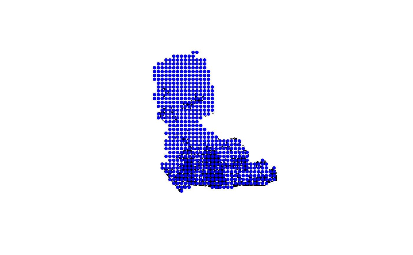
# Radius for AER (meters)
radius_m <- 100

# This function will be dispatched in parallel over computational grids.
aer_at_points <-
  function(
    x, y,
    radius,
    id_col = "pid",
    floors_col = "floors",
    area_col = "foot_m2"
  ) {
    if (!inherits(x, "sf") && !inherits(y, "sf")) {
      x <- sf::st_as_sf(x)
      y <- sf::st_as_sf(y)
    }
    yorig <- y
    y <- sf::st_geometry(y)

    # Buffers around each point
    buf <- sf::st_buffer(y, radius)
    # spatial join (buildings intersecting buffers)
    j <- sf::st_intersects(buf, sf::st_geometry(x))
    # Compute
    out <- vapply(seq_along(j), function(i) {
      if (length(j[[i]]) == 0) return(NA_real_)
      sub <- x[j[[i]], ]
      sub <- sub[!is.na(sub[[floors_col]]) & !is.na(sub[[area_col]]), ]
      if (nrow(sub) == 0) return(NA_real_)
      aer_num <- sum(sub[[area_col]] * sub[[floors_col]], na.rm = TRUE)
      aer_den <- pi * radius^2
      aer_num / aer_den
    }, numeric(1))

    res <-
      data.frame(
        pid = yorig[[id_col]],
        aer = out
      )
    res
  }

## Parallel processing
# Initiate mirai damons
plan(mirai_multisession, workers = 4L)
grd <- chopin::par_pad_grid(
  bldg,
  mode = "grid",
  nx = 1L,
  ny = 4L,
  padding = 300
)

bldg_cast <- sf::st_cast(bldg, "POLYGON")
radius_m <- 300

res <- par_grid_mirai(
  grids    = grd,
  fun_dist = aer_at_points,
  x        = bldg_cast,
  y        = grdpnt,
  radius   = radius_m,
  id_col = "pid",
  .debug = TRUE
)
future::plan(future::sequential)
mirai::daemons(n = 0L)

head(res)
## pid aer
## 1 1 0.2847932
## 2 2 0.7716681
## 3 3 0.4084137
## 4 4 0.4438036
## 5 5 0.6123537
## 6 6 0.5815721Caveats
Why parallelization is slower than the ordinary function run?
- Parallelization may underperform when the datasets are too small to take advantage of divide-and-compute approach, where parallelization overhead is involved. Overhead here refers to the required amount of computational resources for transferring objects to multiple processes.
- Since the demonstrations above use quite small datasets, the advantage of parallelization was not as noticeable as it was expected. Should a large amount of data (spatial/temporal resolution or number of files, for example) be processed, users could find the efficiency of this package. A vignette in this package demonstrates use cases extracting various climate/weather datasets.
Notes on data restrictions
chopin works best with two-dimensional
(planar) geometries. Users should disable
s2 spherical geometry mode in sf by setting
sf::sf_use_s2(FALSE). Running any chopin
functions at spherical or three-dimensional (e.g., including M/Z
dimensions) geometries may produce incorrect or unexpected results.