The coder package simplifies unit classification based
on external code data. this is a generic aim that might be hard to grasp
without further concretization. In this vignette, I will first explain
the overall design principles, and then exemplify the concept with a
typical use case involving patients with total hip arthroplasty (THA)
and their pre-surgery comorbidity. Note, however, that the package is
not limited to patient data or medical settings.
Triad of objects
Functions of the package relies on a triad of objects:
- Case data with unit id:s and possible dates of interest
- External code data for corresponding units in (1) and with optional dates of interest and
- A classification scheme (‘classcodes’ object) with regular expressions to identify and categorize relevant codes from (2).
It is easy to introduce new classification schemes (‘classcodes’
objects) or to use default schemes included in the package (see
vignette("classcodes")).
Triad of functions
There are three important functions to control the intended work flow of the package:
-
codify()will merge object (1) and (2) for a coded data set of the intended format. If optional dates are specified, those will be used to construct time windows in order to filter out only the important dates (i.e. comorbidity during one year before surgery or adverse events 90 days after). -
classify()will then use the coded data and classify it using theclasscodesobject (3) (i.e. to code comorbidity data by the Charlson or Elixhauser comorbidity classifications). -
index()is a third optional step to summarize the individualclasscodescategories to a (possibly weighted) index sum for each coded item (i.e. to calculate the Charlson comorbidity index for each patient).
Those steps could be performed explicitly as
codify() %>% classify() %>% index() or implicitly by
the main function categorize() combining all steps
automatically.
Use case
A typical use case of the coder package would consider
patient data and comorbidity as described in the package readme.
The concept of comorbidity is often attributed to Feinstein (1970):
[T]he term co-morbidity will refer to any distinct additional clinical entity that has existed or that may occur during the clinical course of a patient who has the index disease under study.
Let’s consider a group of patients with THA, as identified from a national quality register, which might be large in size. Assume we are interested in those patients’ pre-surgery comorbidity, which is not captured by the quality register itself. Instead, this data might be codified in a secondary source, such as a national patient register containing all hospital visits and admissions during several years, both before and after the THA-surgery. Each hospital visit/admission might be recorded with one or several medical codes, for example using the International classification of diseases version 10 (ICD-10). Similarly, a medical prescription register might hold records of prescribed drugs with their corresponding codes from the Anatomic therapeutic chemical classification (ATC) system.
Thus, combining the primary and secondary data sets (objects 1-2
above) using some unique patient id, and a possible time window (i.e. to
only consider comorbidity as recorded during one year before the THA),
is a first step to identify patient comorbidity. This step is performed
by the codify() function in step (i) above.
We have now gathered all the relevant codes for each patient. Common
classifications (i.e. ICD-10 and ATC) are wast, however, including tens
of thousands of medical/chemical codes, which are cumbersome and
impractical to use directly. It is therefore common to categorize such
codes into broader categories (i.e. by the Charlson, Elixhauser or
RxRisk V classifications as below). Such classification could be a
simple code matching problem using a look-up table. This is generally a
slow, cumbersome and error-prone process, however. I therefore recommend
to use regular expression for a compact code representation, as well as
a computationally faster procedure. This is implemented in the
classify() function from step (ii) above.
We have now reduced the data from tens of thousands of codes to
perhaps 10-50 combined categories. This might be sufficient in some
cases, although further simplifications might also be needed. It is thus
common to simplify comorbidity into a single number, an index score, as
the sum of individual comorbidities, possible weighted to differentiate
more serious conditions from more trivial. Different weights might be of
relevance under different circumstances or in different fields. This is
implemented by the index() function in step (iii)
above.
Charlson and Elixhauser
The Charlson (1987) and Elixhauser (1998) comorbidity indices are two examples used in medical research. Each index consist of several medical conditions, possibly summarized by a (weighted) index. Each condition is defined by a set of medical codes (Quan et al. 2005). Different versions of the International Classification of Diseases (ICD) codes are often used.
The coder package provides substantial functionality for
both Charlson and Elixhauser, although we will not focus on those
indices here (but see examples in vignette("classcodes")).
Several other R packages have functions for Charlson and Elixhauser:
icd and comorbidity are both good packages
well suited for their purpose based on effective implementations.
medicalrisk can be used with ICD-9-CM codes but is not
up-to-date with the latest version of ICD-10.
comorbidities.icd10 and icdcoder are not
actively developed or maintained.
One advantage with the coder package is the great
flexibility for combining different sets of codes (ICD-8, ICD-9,
ICD-9-CM and ICD-10 et cetera), with different weighted indices.
Risk Rx V
Another advantage of the coder package is the inclusion
of additional classifications (see ?all_classcodes()), such
as the pharmacy-based case-mix instrument Rx Risk V (Sloan et al. 2003). We will use this
classification in an example. This classification, in contrast to
Charlson and Elixhauser, relies on medical prescription data codified by
the Anatomic Therapeutic Chemical classification system (ATC).
As for all classcodes objects in the package, additional information
and references are found in the object documentation
(?rxriskv).
Concrete example
Let us consider the hypothetical setting above using some example
data (ex_peopple and ex_atc) as described in
vignette("ex_data").
Default categorization
A first attempt to calculate the Rx Risk V score for each patient:
default <- categorize(
    ex_people, codedata = ex_atc, cc = rxriskv, id = "name", code = "atc")
#> Classification based on: atc_pratt
default
#> # A tibble: 100 × 50
#>    name     surgery    Alcohol.dependence Allergies Anticoagulants Antiplatelets
#>    <chr>    <date>     <lgl>              <lgl>     <lgl>          <lgl>
#>  1 Chen, T… 2025-04-21 FALSE              TRUE      TRUE           FALSE
#>  2 Graves,… 2025-01-11 FALSE              FALSE     FALSE          FALSE
#>  3 Trujill… 2024-12-29 FALSE              FALSE     FALSE          FALSE
#>  4 Simpson… 2025-04-02 FALSE              TRUE      FALSE          FALSE
#>  5 Chin, N… 2025-03-16 FALSE              FALSE     FALSE          TRUE
#>  6 Le, Chr… 2024-10-18 FALSE              FALSE     FALSE          FALSE
#>  7 Kang, X… 2025-01-20 FALSE              TRUE      FALSE          TRUE
#>  8 Shuemak… 2024-10-19 FALSE              FALSE     FALSE          FALSE
#>  9 Boucher… 2025-03-27 FALSE              FALSE     FALSE          FALSE
#> 10 Le, Sor… 2025-03-01 FALSE              FALSE     FALSE          FALSE
#> # ℹ 90 more rows
#> # ℹ 44 more variables: Anxiety <lgl>, Arrhythmia <lgl>,
#> #   Benign.prostatic.hyperplasia <lgl>, Bipolar.disorder <lgl>,
#> #   Chronic.airways.disease <lgl>, Congestive.heart.failure <lgl>,
#> #   Dementia <lgl>, Depression <lgl>, Diabetes <lgl>, Epilepsy <lgl>,
#> #   Gastrooesophageal.reflux.disease <lgl>, Glaucoma <lgl>, Gout <lgl>,
#> #   Hepatitis.B <lgl>, Hepatitis.C <lgl>, HIV <lgl>, Hyperkalaemia <lgl>, …
The first two columns are identical to ex_people.
Additional columns indicate whether patients had any of the individual
comorbidities identified by Rx Risk V. Patients without any medical
prescriptions have NA values (which might be substituted by
FALSE). The last columns contain summarized index values
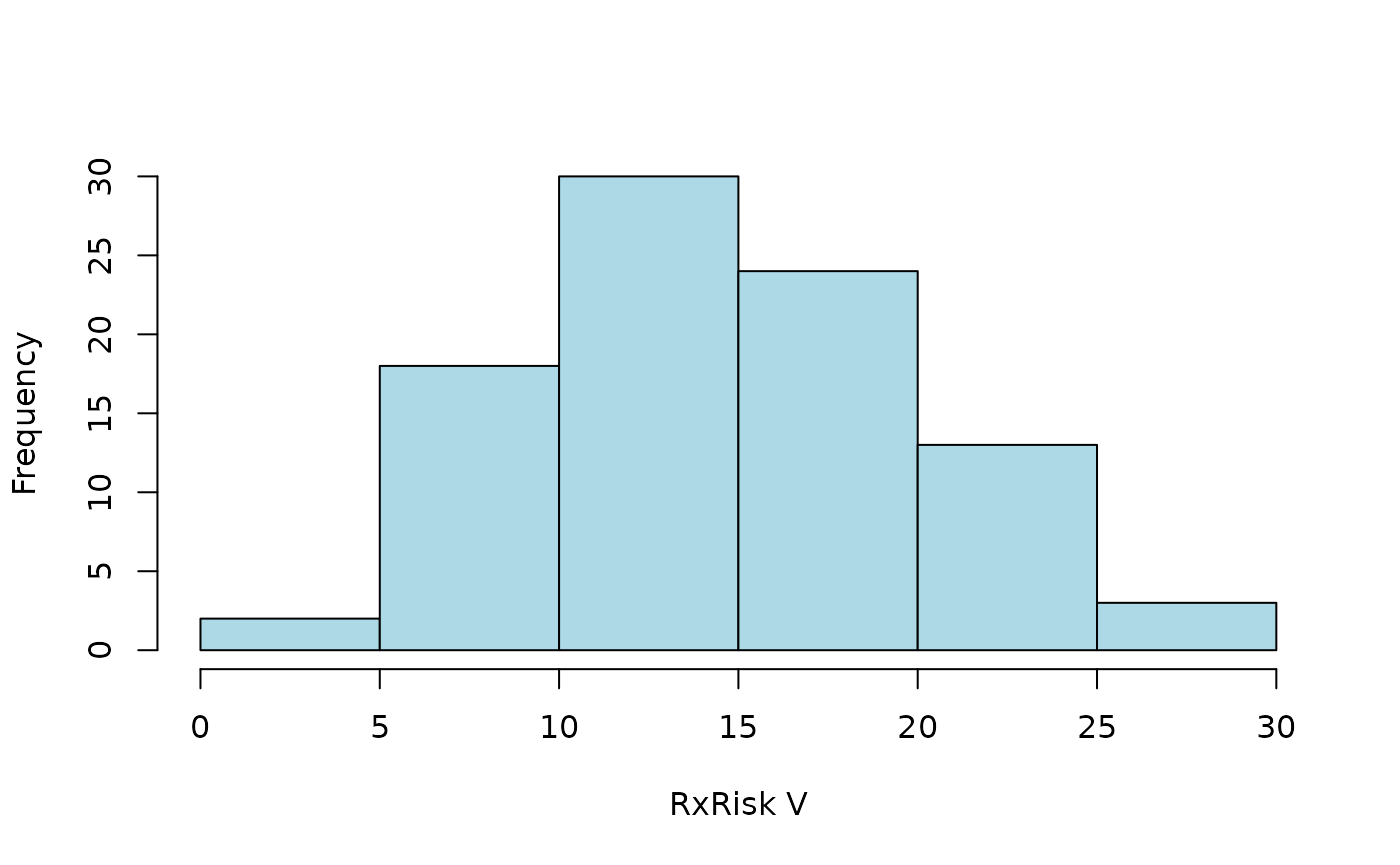
(weighted sums of individual comorbidities). Let’s summarize the
distribution of a weighted index according to pratt (Pratt et al. 2018):
hist2 <- function(x) {
  hist(x$pratt, main = NULL, xlab = "RxRisk V", col = "lightblue")
}
hist2(default)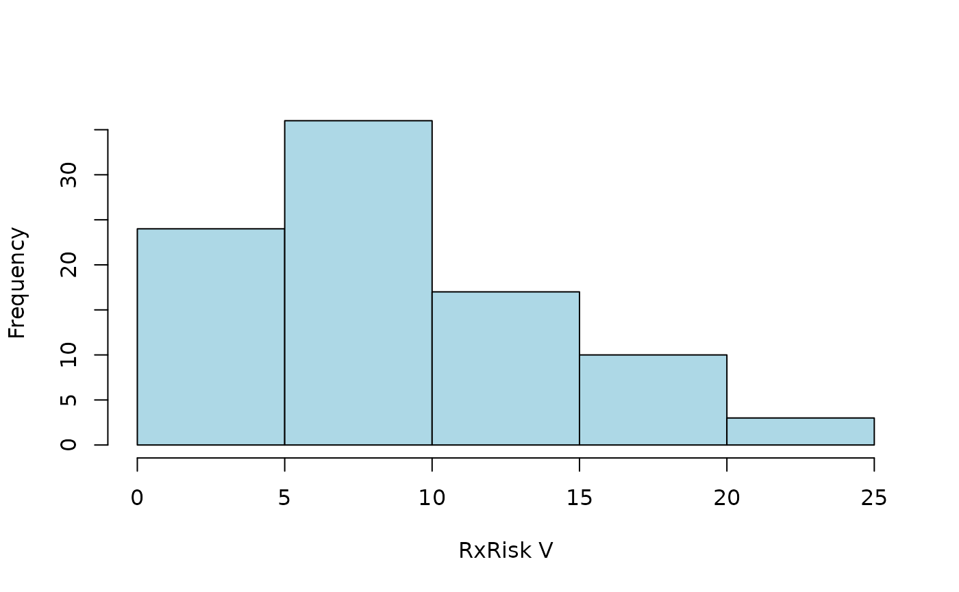
Specified time-window
Some prescriptions might have been filed long before surgery, or even
after. Those codes are less relevant for comorbidities present at
surgery. We can limit the categorization to a time window of one year
(365 days) prior to surgery. This is done internally by the
codify() function, hence by specifying a list of arguments
passed to this function:
codify_args <-
  list(date = "surgery", code_date = "prescription", days = c(-365, -1))

ct <-
  categorize(
    ex_people,
    codedata    = ex_atc,
    cc          = rxriskv,
    id          = "name",
    code        = "atc",
    codify_args = codify_args
  )
#> Classification based on: atc_pratt

hist2(ct)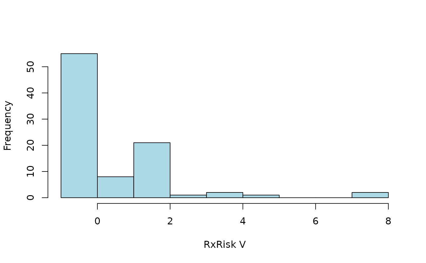
Alternative classification
Comorbidities are identified from ATC codes captured by regular
expression (see vignette("classcodes") and
vignette("Intrpret_regular_expressions")). Codes identified
by atc_pratt are used by default. Let’s use an alternative
version adopted from Caughy (2010) as
specified by an argument passed by the cc_args
argument.
hist2(
  categorize(
    ex_people,
    codedata      = ex_atc,
    cc            = rxriskv,
    id            = "name",
    code          = "atc",
    codify_args   = codify_args,
    cc_args       = list(regex = "caughey")
  )
)
Specified index
We did not specify how to calculate the weighted index sum above,
wherefore all available indices were provided by default. We might go
back to Pratt’s classification scheme (atc_pratt) and only
calculate the corresponding index pratt. Let´s also perform
the three computational steps explicitly instead of using the combining
categorize() function and tabulate the result
codify(
  ex_people,
  ex_atc,
  id        = "name",
  code      = "atc",
  date      = "surgery",
  code_date = "prescription",
  days      = c(-365, -1)
) %>%
  classify(rxriskv) %>%
  index("pratt") %>%
  table()
#> Warning: 'classify()' does not preserve row order ('categorize()' does!)
#> Classification based on: atc_pratt
#> .
#> -1  0  1  2  3  4  5  8
#> 12 43  8 21  1  2  1  2
Dirty code data
Let’s assume that our code data is not as clean as simulated above.
s <- function(x) sample(x, 1e3, replace = TRUE)

ex_atc$code <-
  paste0(
    s(letters), s(0:9), s(letters), s(c(".", "-", "?")),
    ex_atc$atc, s(letters), s(0:9)
  )

ex_atc
#> # A tibble: 10,000 × 4
#>    name                 atc      prescription code
#>    <chr>                <chr>    <date>       <chr>
#>  1 Le, Soraiya          L03AA16  2023-01-23   m5g.L03AA16h7
#>  2 Cleveland, Mark      J07CA01  2020-10-02   w3p.J07CA01m1
#>  3 Santistevan, Charlie QJ57EA06 2016-03-13   l3d.QJ57EA06f2
#>  4 Meier, Hayden        R03DB04  2021-07-14   e8o-R03DB04s5
#>  5 Hill, Audrey         V09IA01  2018-12-27   f3s.V09IA01s1
#>  6 Thumma, Phillip      L02AE02  2015-02-04   o8j?L02AE02t3
#>  7 Yost, Rebecca        S01EB06  2019-06-29   o8j?S01EB06r7
#>  8 Mandakh, Joseph      A03DA01  2021-01-30   d7w-A03DA01k8
#>  9 Meier, Hayden        C09AA13  2023-07-22   f3n-C09AA13m5
#> 10 Trinh, Schuyler      A07EA03  2025-05-21   i7r?A07EA03n8
#> # ℹ 9,990 more rows

sum(
  categorize(
    ex_people,
    codedata = ex_atc,
    cc       = rxriskv,
    id       = "name",
    code     = "code"
  )$pratt,
  na.rm      = TRUE
)
#> Classification based on: atc_pratt
#> [1] 0
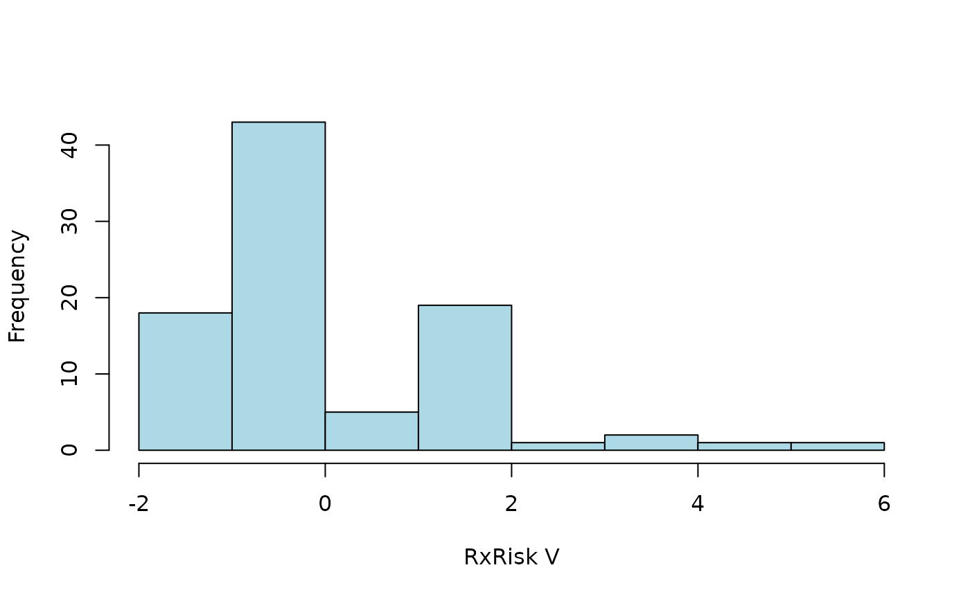
Thus, no codes are recognized (every one got index = 0). By default,
codes are only recognized if found immediate in its corresponding
column. This can be controlled by arguments start and
stop specified via cc_args. We can also ignore
all non alphanumeric characters by setting alnum = TRUE as
passed to codify() by argument
codify_args.
hist2(
  categorize(
    ex_people,
    codedata = ex_atc,
    cc       = rxriskv,
    id       = "name",
    code     = "code",
    cc_args  = list(
      start  = FALSE,
      stop   = FALSE
    ),
    codify_args = list(
      alnum = TRUE
    )
  )
)
#> Classification based on: atc_pratt