dendroNetwork is a package to create dendrochronological networks for gaining insight into provenance or other patterns based on the statistical relations between tree ring curves. The code and the functions are based on several published papers (Visser 2021b, 2021a; Visser and Vorst 2022).
The package is written for dendrochronologists and have a general knowledge on the discipline and used jargon. There is an excellent website for the introduction of using R in dendrochronology: https://opendendro.org/r/. The basics of dendrochronology can be found in handbooks (Cook and Kariukstis 1990; Speer 2010) or on https://www.dendrohub.com/. A list of R-packages for dendrochronology can be found here: https://ronaldvisser.github.io/Dendro_R/.
Installation
This package depends on RCy3, which is part of Bioconductor. Therefore it is recommended to install RCy3 first using:
if (!require("BiocManager", quietly = TRUE))
    install.packages("BiocManager")

BiocManager::install("RCy3")
The functionality of RCy3 depends on the installation of Cytoscape. Cytoscape is needed for visualising the networks. This open source software is platform independent and provides easy visual access to complex networks and the attributes of both nodes and edges in a network (see the Cytoscape-website for more information). It is therefore recommended to install Cytoscape as well. Please follow the download and installation instructions for your operating system: https://cytoscape.org/.
You can install the latest version of dendroNetwork from CRAN or the development version from R-universe by running one of the commands below:
# CRAN
install.packages("dendroNetwork")
# R-Universe
install.packages("dendroNetwork", repos = "https://ropensci.r-universe.dev")
Usage
The package aims to make the creation of dendrochronological (provenance) networks as easy as possible. To be able to make use of all options, it is assumed that Cytoscape (Shannon et al. 2003)is installed (https://cytoscape.org/). Some data is included in this package, namely the Roman data published by Hollstein (Hollstein 1980).
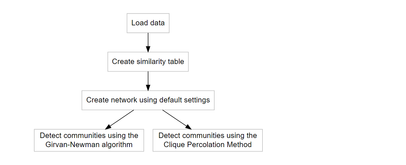
The first steps are visualized in the flowchart below, including community detection using either (or both) the Girvan-Newman algorithm (Girvan and Newman 2002) and Clique Percolation Method (Palla et al. 2005) for all clique sizes. Both methods are explained very well in the papers, and on wikipedia for both CPM and the Girvan-Newman algorithm.
library(dendroNetwork)
data(hol_rom) # 1
sim_table_hol <- sim_table(hol_rom) # 2
g_hol <- dendro_network(sim_table_hol) # 3
g_hol_gn <- gn_names(g_hol) # 4
g_hol_cpm <- clique_community_names(g_hol, k=3) # 4
hol_com_cpm_all <- find_all_cpm_com(g_hol) # 5
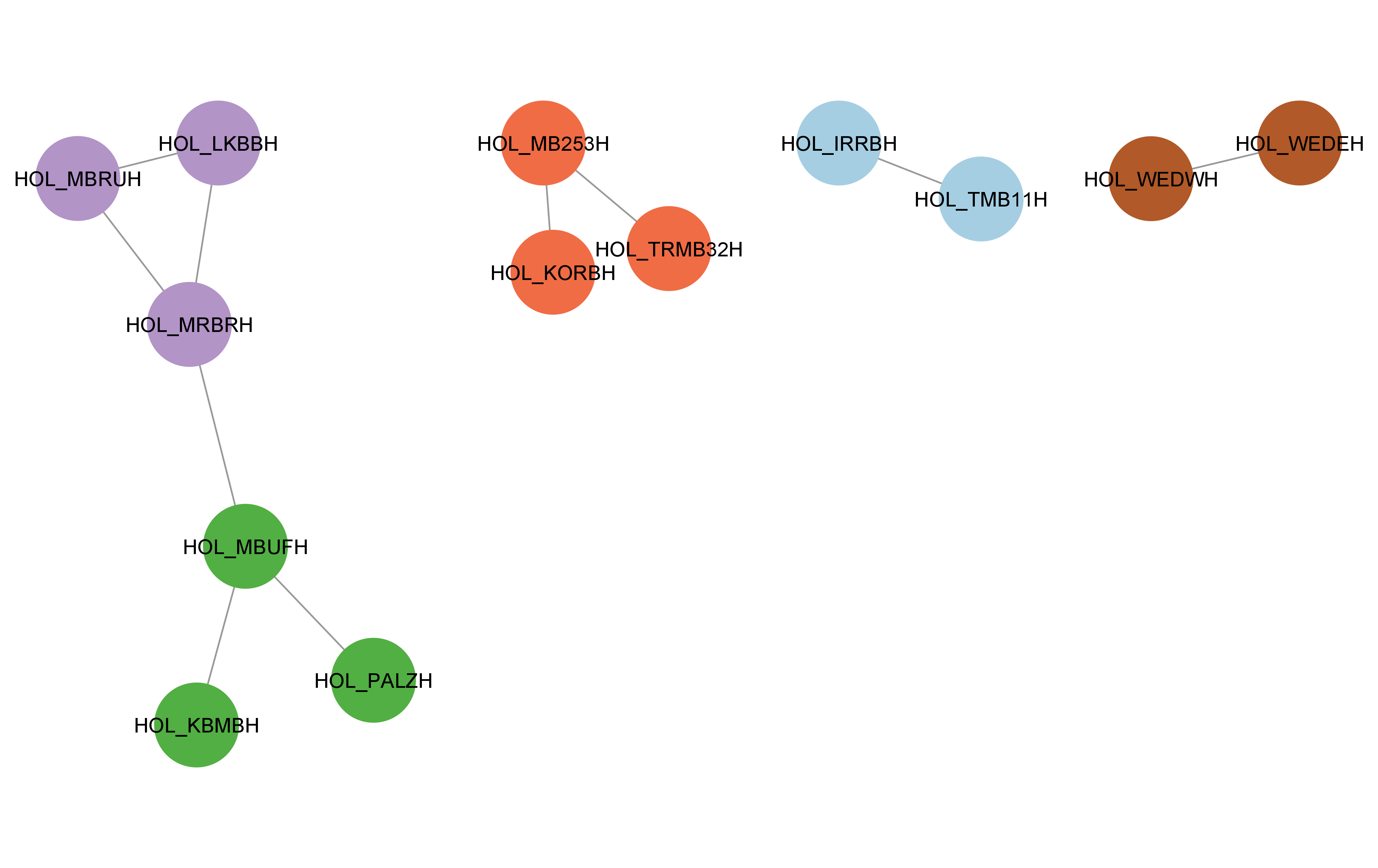
plot(g_hol) # plotting the graph in R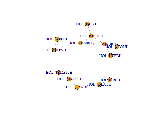
plot(g_hol, vertex.color="deepskyblue", vertex.size=15, vertex.frame.color="gray",
     vertex.label.color="darkslategrey", vertex.label.cex=0.8, vertex.label.dist=2) # better readable version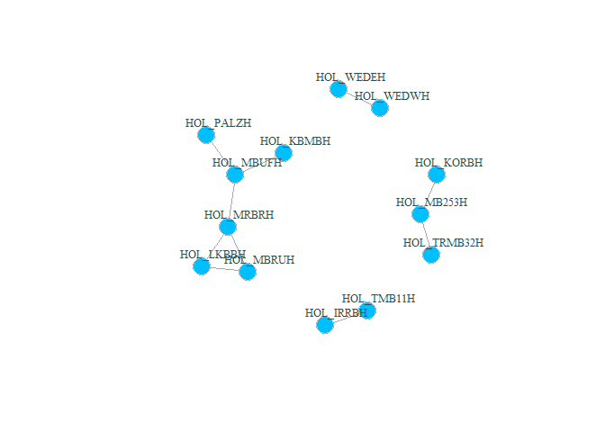
Visualization in Cytoscape
After creating the network in R, it is possible to visualize the network using Cytoscape. The main advantage is that visualisation in Cytoscape is more easy, intuitive and visual. In addition, it is very easy to automate workflows in Cytoscape with R (using RCy3). For this purpose we need to start Cytoscape firstly. After Cytoscape has completely loaded, the next steps can be taken.
- The network can now be loaded in Cytoscape for further visualisation:
cyto_create_graph(g_hol, CPM_table = hol_com_cpm_all, GN_table = g_hol_gn) - Styles for visualisation can now be generated. However, Cytoscape comes with a lot of default styles that can be confusing. Therefore it is recommended to use:
cyto_clean_styles()once in a session. - To visualize the styles for CPM with only k=3:
cyto_create_cpm_style(g_hol, k=3, com_k = g_hol_cpm)- This can be repeated for all possible clique sizes. To find the maximum clique size in a network, please use:
igraph::clique_num(g_hol). - To automate this:
for (i in 3:igraph::clique_num(g_hol)) { cyto_create_cpm_style(g_hol, k=i, com_k = g_hol_cpm)}.
- This can be repeated for all possible clique sizes. To find the maximum clique size in a network, please use:
- To visualize the styles using the Girvan-Newman algorithm (GN):
cyto_create_gn_style(g_hol)This would look something like this in Cytoscape:
Usage for large datasets
When using larger datasets of tree-ring series, calculating the table with similarities can take a lot of time, but finding communities even more. It is therefore recommended to use of parallel computing for Clique Percolation: clique_community_names_par(network, k=3, n_core = 4). This reduces the amount of time significantly. For most datasets clique_community_names() is sufficiently fast and for smaller datasets clique_community_names_par() can even be slower due to the parallelisation. Therefore, the function clique_community_names() should be used initially and if this is very slow, start using clique_community_names_par(). See the separate vignette for that.
Citation
If you use this software, please cite this using:
Visser, R.M. (2025). dendroNetwork: a R-package to create dendrochronological provenance networks (Version 0.5.5) [Computer software]. https://zenodo.org/doi/10.5281/zenodo.10636310
Acknowledgements
This package reuses and adapts the CliquePercolationMethod-R package developed by Angelo Salatino (The Open University). Source code: https://github.com/angelosalatino/CliquePercolationMethod-R
This package reuses and adapts the function cor.with.limit.R() developed by Andy Bunn (Western Washington University), but the new function is optimized and also outputs the number of overlapping rings. Source code: https://github.com/AndyBunn/dplR/blob/master/R/rwi.stats.running.R.