Storing Large Dataframes

Thierry Onkelinx

Introduction

Sometimes, a large dataframe has one or more variables with a small number of unique combinations. E.g. a dataframe with one or more factor variables. Storing the entire dataframe as a single text file requires storing lots of replicated data. Each row stores the information for every variable, even if a subset of these variables remains constant over a subset of the data.

In such a case we can use the split_by argument of write_vc(). This will store the large dataframe over a set of tab separated files. One file for every combination of the variables defined by split_by. Every partial data file holds the other variables for one combination of split_by. We remove the split_by variables from the partial data files, reducing their size. We add an index.tsv containing the combinations of the split_by variables and a unique hash for each combination. This hash becomes the base name of the partial data files.

Splitting the dataframe into smaller files makes them easier to handle in version control system. The total size depends on the amount of replication in the dataframe. More on that in the next section.

When to Split the Dataframe

Let’s set the following variables:

• $s$: the average number of bytes to store a single line of the split_by variables.

• $r$: the average number of bytes to store a single line of the remaining variables.

• $h_s$: the number of bytes to store the header of the split_by variables.

• $h_r$: the number of bytes to store the header of the remaining variables.

• $N$: the number of rows in the dataframe.

• $N_s$: the number of unique combinations of the split_by variables.

Storing the dataframe with write_vc() without split_by requires $h_s + h_r + 1$ bytes for the header and $s + r + 1$ bytes for every observation. The total number of bytes is $T_0 = h_s + h_r + 1 + N (s + r + 1)$. Both $+ 1$ originate from the tab character to separate the split_by variables from the remaining variables.

Storing the dataframe with write_vc() with split_by requires an index file to store the combinations of the split_by variables. It will use $h_s$ bytes for the header and $N_s s$ for the data. The headers of the partial data files require $N_s h_r$ bytes ($N_s$ files and $h_r$ byte per file). The data in the partial data files require $N r$ bytes. The total number of bytes is $T_s = h_s + N_s s + N_s h_r + N r$.

We can look at the ratio of $T_s$ over $T_0$.

$$\frac{T_s}{T_0} = \frac{h_s + N_s s + N_s h_r + N r}{h_s + h_r + 1 + N (s + r + 1)}$$

Let’s simplify the equation by assuming that we need an equal amount of character for the headers and the data ($h_s = s$ and $h_r = r$).

$$\frac{T_s}{T_0} = \frac{s + N_s s + N_s r + N r}{s + r + 1 + N (s + r + 1)}$$

$$\frac{T_s}{T_0} = \frac{s + N_s s + N_s r + N r}{s + r + 1 + N s + N r + N}$$

Let assume that $s = a r$ with $0 < a$ and $N_s = b N$ with $0 < b < 1$.

$$\frac{T_s}{T_0} = \frac{a r + N a b r + N b r + N r}{a r + r + 1 + N a r + N r + N}$$

$$\frac{T_s}{T_0} = \frac{(a + N a b + N b + N) r}{(N + 1) (a r + r + 1)}$$

$$\frac{T_s}{T_0} = \frac{a + N a b + N b + N}{(N + 1) (a + 1 + 1 / r)}$$$$\frac{T_s}{T_0} = \frac{a + (a b + b + 1) N }{(N + 1) (a + 1 + 1 / r)}$$

When $N$ is large, we can state that $a \lll N$ and $N / (N + 1) \approx 1$.

$$\frac{T_s}{T_0} \approx \frac{a b + b + 1}{a + 1 + 1 / r}$$

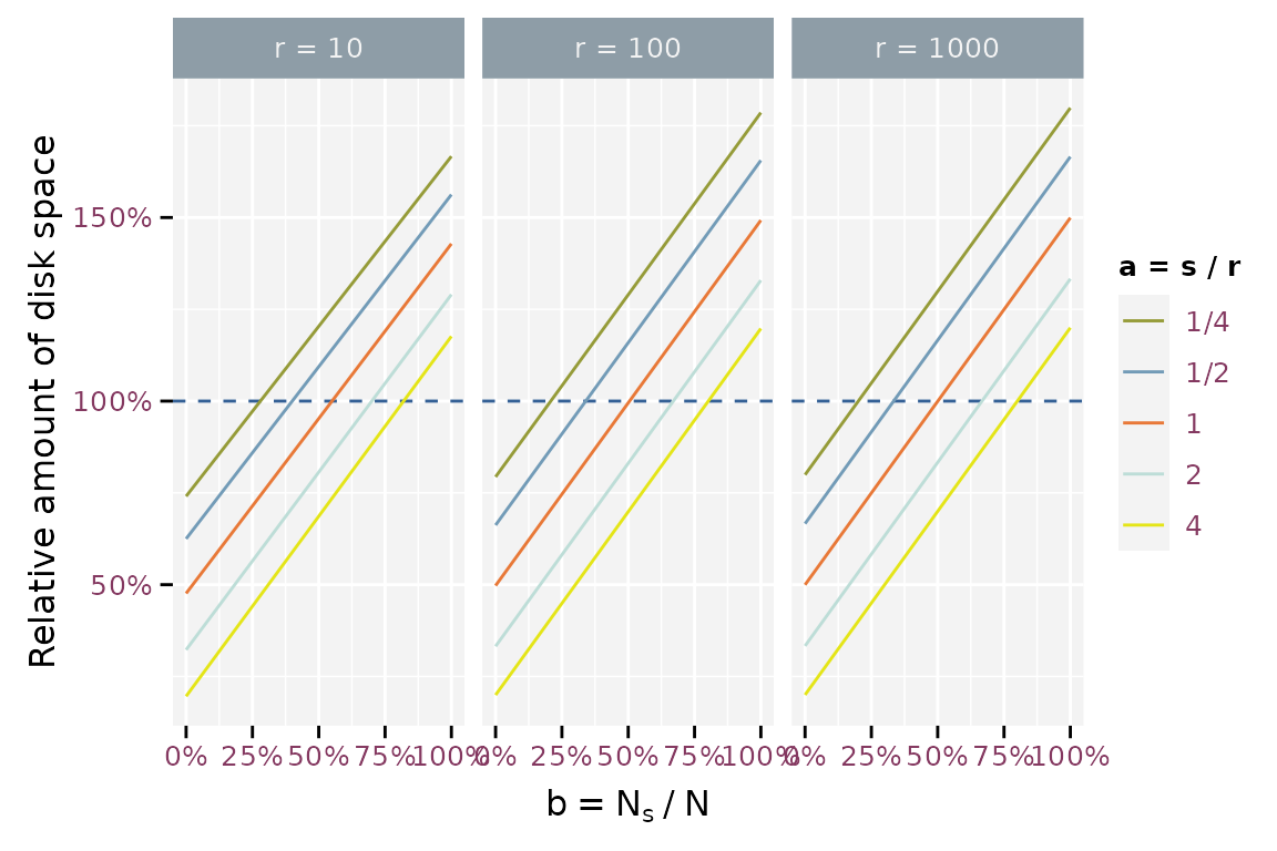
Storage space required using split_by relative to storing a single file.

The figure illustrates that using split_by is more efficient when the number of unique combinations ($N_s$) of the split_by variables is much smaller than the number of rows in the dataframe ($N$). The efficiency also increases when the storage for a single combination of split_by variables ($s$) is larger than the storage needed for a single line of the remain variables ($r$). The storage needed for a single line of the remain variables ($r$) doesn’t influence the efficiency.

Benchmarking

library(git2rdata)
root <- tempfile("git2rdata-split-by")
dir.create(root)

library(microbenchmark)
mb <- microbenchmark(
  part_1 = write_vc(airbag, "part_1", root, sorting = "X"),
  part_2 = write_vc(airbag, "part_2", root, sorting = "X", split_by = "airbag"),
  part_3 = write_vc(airbag, "part_3", root, sorting = "X", split_by = "abcat"),
  part_4 = write_vc(
    airbag, "part_4", root, sorting = "X", split_by = c("airbag", "sex")
  ),
  part_5 = write_vc(airbag, "part_5", root, sorting = "X", split_by = "dvcat"),
  part_6 = write_vc(
    airbag, "part_6", root, sorting = "X", split_by = "yearacc"
  ),
  part_15 = write_vc(
    airbag, "part_15", root, sorting = "X", split_by = c("dvcat", "abcat")
  ),
  part_45 = write_vc(
    airbag, "part_45", root, sorting = "X", split_by = "yearVeh"
  ),
  part_270 = write_vc(
    airbag, "part_270", root, sorting = "X", split_by = c("yearacc", "yearVeh")
  )
)
mb$time <- mb$time / 1e6

Splitting the dataframe over more than one file takes more time to write the data. The log time seems to increase quadratic with log number of parts.

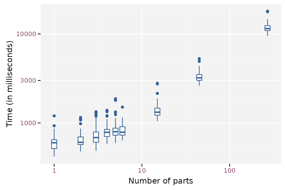
Boxplot of the write timings for different number of parts.

mb_r <- microbenchmark(
  part_1 = read_vc("part_1", root),
  part_2 = read_vc("part_2", root),
  part_3 = read_vc("part_3", root),
  part_4 = read_vc("part_4", root),
  part_5 = read_vc("part_5", root),
  part_6 = read_vc("part_6", root),
  part_15 = read_vc("part_15", root),
  part_45 = read_vc("part_45", root),
  part_270 = read_vc("part_270", root)
)
mb_r$time <- mb_r$time / 1e6

A small number of parts does not seem to affect the read timings much. Above ten parts, the required time for reading seems to increase. The log time seems to increase quadratic with log number of parts.

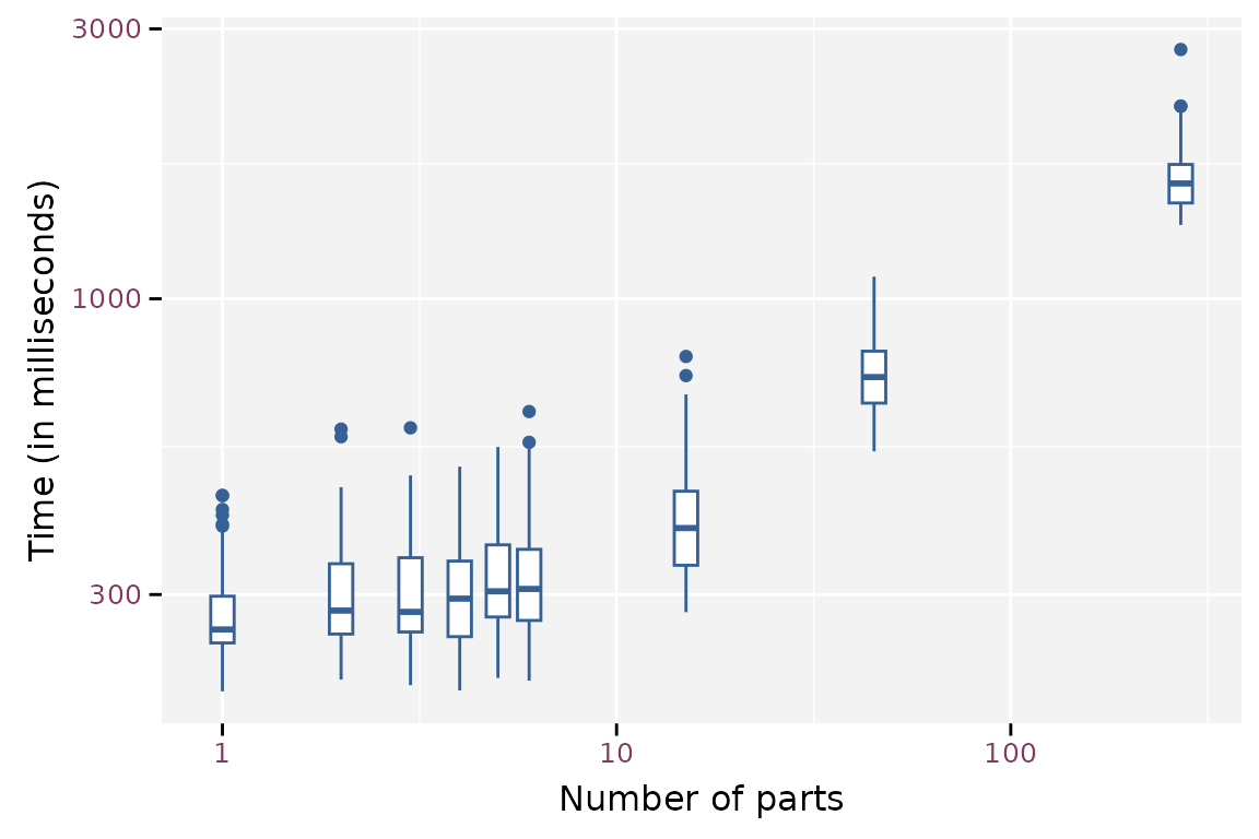
Boxplot of the read timings for the different number of parts.