Efficiency Relative to Storage and Time

Introduction

This vignette compares storage and retrieval of data by git2rdata with other standard R functionality. We consider write.table() and read.table() for data stored in a plain text format. saveRDS() and readRDS() use a compressed binary format.

To get some meaningful results, we will use the nassCDS dataset from the DAAG package. We’ll avoid the dependency on the package by directly downloading the data.

airbag <- read.csv(
  "https://vincentarelbundock.github.io/Rdatasets/csv/DAAG/nassCDS.csv"
)
airbag$dead <- airbag$dead == "dead"
airbag$airbag <- airbag$airbag == "airbag"
airbag$seatbelt <- airbag$seatbelt == "belted"
airbag$dvcat <- as.ordered(airbag$dvcat)

str(airbag)
#> 'data.frame':    26217 obs. of  16 variables:
#>  $ X          : int  1 2 3 4 5 6 7 8 9 10 ...
#>  $ dvcat      : Ord.factor w/ 5 levels "1-9km/h"<"10-24"<..: 3 2 2 3 3 4 5 5 2 2 ...
#>  $ weight     : num  25.1 25.1 32.4 495.4 25.1 ...
#>  $ dead       : logi  FALSE FALSE FALSE FALSE FALSE FALSE ...
#>  $ airbag     : logi  FALSE TRUE FALSE TRUE FALSE FALSE ...
#>  $ seatbelt   : logi  TRUE TRUE FALSE TRUE TRUE TRUE ...
#>  $ frontal    : int  1 1 1 1 1 1 1 1 0 1 ...
#>  $ sex        : Factor w/ 2 levels "f","m": 1 1 1 1 1 1 2 2 2 1 ...
#>  $ ageOFocc   : int  26 72 69 53 32 22 22 32 40 18 ...
#>  $ yearacc    : int  1997 1997 1997 1997 1997 1997 1997 1997 1997 1997 ...
#>  $ yearVeh    : int  1990 1995 1988 1995 1988 1985 1984 1987 1984 1987 ...
#>  $ abcat      : Factor w/ 3 levels "deploy","nodeploy",..: 3 1 3 1 3 3 3 3 3 3 ...
#>  $ occRole    : Factor w/ 2 levels "driver","pass": 1 1 1 1 1 1 1 1 1 1 ...
#>  $ deploy     : int  0 1 0 1 0 0 0 0 0 0 ...
#>  $ injSeverity: int  3 1 4 1 3 3 3 4 1 0 ...
#>  $ caseid     : Factor w/ 9409 levels "11:1:1","11:1:2",..: 1645 1646 1688 1488 1510 1511 1555 1556 1571 1572 ...

Data Storage

On a File System

We start by writing the dataset as is with write.table(), saveRDS(), write_vc() and write_vc() without storage optimization. Note that write_vc() uses optimization by default. Since write_vc() creates two files for each data set, we take their combined file size into account.

library(git2rdata)
root <- tempfile("git2rdata-efficient")
dir.create(root)

write.table(airbag, file.path(root, "base_R.tsv"), sep = "\t")
base_size <- file.size(file.path(root, "base_R.tsv"))

saveRDS(airbag, file.path(root, "base_R.rds"))
rds_size <- file.size(file.path(root, "base_R.rds"))

fn <- write_vc(airbag, "airbag_optimize", root, sorting = "X")
optim_size <- sum(file.size(file.path(root, fn)))

fn <- write_vc(airbag, "airbag_verbose", root, sorting = "X", optimize = FALSE)
verbose_size <- sum(file.size(file.path(root, fn)))

Since the data is highly compressible, saveRDS() yields the smallest file at the cost of having a binary file format. Both write_vc() formats yield smaller files than write.table(). Partly because write_vc() doesn’t store row names and doesn’t use quotes unless needed. The difference between the optimized and verbose version of write_vc() is, in this case, solely due to the way write_vc() stores factors in the data (tsv) file. The optimized version stores the indices of the factor whereas the verbose version stores the levels. For example: airbag$dvcat has 5 levels with short labels (on average 5 character), storing the index requires 1 character. This results in more compact files.

Resulting file sizes (in kB) and file sizes relative to the size of write.table().
method	file_size	relative
saveRDS()	313.13	0.12
write_vc(), optimized	1739.99	0.64
write_vc(), verbose	2467.19	0.91
write.table()	2716.93	1.00

The reduction in file size when storing in factors depends on the length of the labels, the number of levels and the number of observations. The figure below illustrates the strong gain as soon as the level labels contain more than two characters. The gain is less pronounced when the factor has a large number of levels. The optimization fails in extreme cases with short factor labels and a high number of levels.

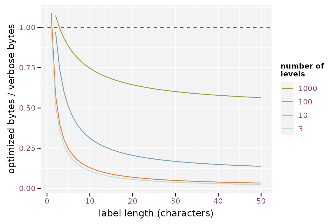
Effect of the label length on the efficiency of storing factor optimized, assuming 1000 observations

The effect of the number of observations is mainly due to the overhead of storing the metadata. The importance of this overhead increases when the number of observations is small.

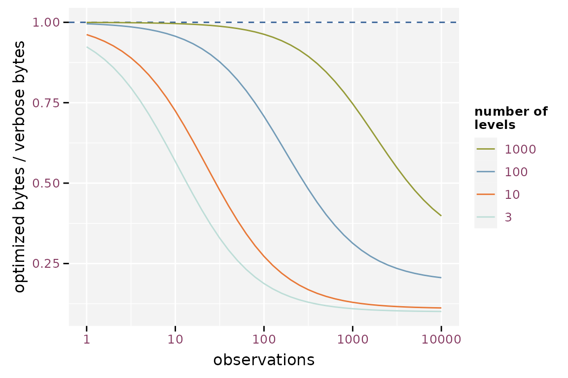
Effect of the number of observations on the efficiency of storing factor optimized assuming labels with 10 characters

In Git Repositories

Here we will simulate how much space the data requires to store the history in a git repository. We will create a git repository for each method and store different subsets of the same data. Each commit contains a new version of the data. Each version is a random sample containing 90% of the observations of the airbag data. Two consecutive versions of the subset will have about 90% of the observations in common.

After writing each version, we commit the file, perform garbage collection (git gc) on the git repository and then calculate the size of the git history (git count-objects -v).

library(git2r)
tmp_repo <- function() {
  root <- tempfile("git2rdata-efficient-git")
  dir.create(root)
  repo <- git2r::init(root)
  git2r::config(repo, user.name = "me", user.email = "me@me.com")
  return(repo)
}
commit_and_size <- function(repo, filename) {
  add(repo, filename)
  commit(repo, "test", session = TRUE)
  git_size <- system(
    sprintf("cd %s\ngit gc\ngit count-objects -v", dirname(repo$path)),
    intern = TRUE
  )
  git_size <- git_size[grep("size-pack", git_size)]
  as.integer(gsub(".*: (.*)", "\\1", git_size))
}

repo_wt <- tmp_repo()
repo_wts <- tmp_repo()
repo_rds <- tmp_repo()
repo_wvco <- tmp_repo()
repo_wvcv <- tmp_repo()

repo_size <- replicate(
  100, {
    observed_subset <- rbinom(nrow(airbag), size = 1, prob = 0.9) == 1
    this <- airbag[
      sample(which(observed_subset)),
      sample(ncol(airbag))
    ]
    this_sorted <- airbag[observed_subset, ]
    fn_wt <- file.path(workdir(repo_wt), "base_R.tsv")
    write.table(this, fn_wt, sep = "\t")
    fn_wts <- file.path(workdir(repo_wts), "base_R.tsv")
    write.table(this_sorted, fn_wts, sep = "\t")
    fn_rds <- file.path(workdir(repo_rds), "base_R.rds")
    saveRDS(this, fn_rds)
    fn_wvco <- write_vc(this, "airbag_optimize", repo_wvco, sorting = "X")
    fn_wvcv <- write_vc(
      this, "airbag_verbose", repo_wvcv, sorting = "X", optimize = FALSE
    )
    c(
      write.table = commit_and_size(repo_wt, fn_wt),
      write.table.sorted = commit_and_size(repo_wts, fn_wts),
      saveRDS = commit_and_size(repo_rds, fn_rds),
      write_vc.optimized = commit_and_size(repo_wvco, fn_wvco),
      write_vc.verbose = commit_and_size(repo_wvcv, fn_wvcv)
    )
})

Each version of the data has on purpose a random order of observations and variables. This is what would happen in a worst case scenario as it would generate the largest possible diff. We also test write.table() with a stable ordering of the observations and variables.

The randomised write.table() yields the largest git repository, converging to about 6.5 times the size of a git repository based on the sorted write.table(). saveRDS() yields a 26% reduction in repository size compared to the randomised write.table(), but still is 4.8 times larger than the sorted write.table(). Note that the gain of storing binary files in a git repository is much smaller than the gain in individual file size because git compresses its history. The optimized write_vc() starts at 88% and converges toward 78%, the verbose version starts at 94% and converges towards 110%. Storage size is a lot smaller when using write_vc() with optimization. The verbose option of write_vc() has little the gain in storage size. Another advantage is that write_vc() stores metadata.

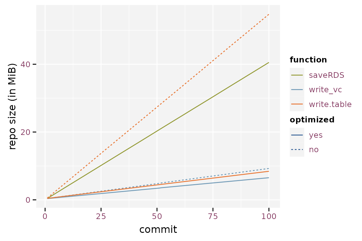
Size of the git history using the different storage methods.

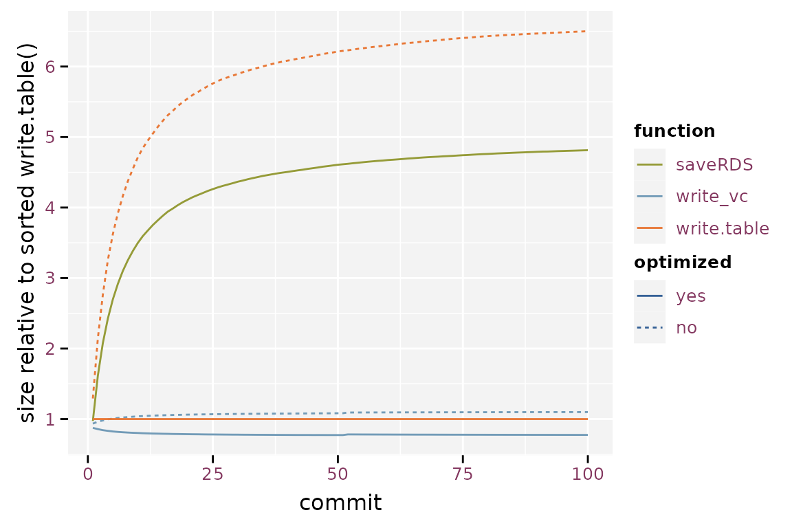
Relative size of the git repository when compared to write.table().

Timings

The code below runs a microbenchmark on the four methods. A microbenchmark runs the code a hundred times and yields a distribution of timings for each expression.

Writing Data

library(microbenchmark)
mb <- microbenchmark(
  write.table = write.table(airbag, file.path(root, "base_R.tsv"), sep = "\t"),
  saveRDS = saveRDS(airbag, file.path(root, "base_R.rds")),
  write_vc.optim = write_vc(airbag, "airbag_optimize", root, sorting = "X"),
  write_vc.verbose = write_vc(airbag, "airbag_verbose", root, sorting = "X",
                              optimize = FALSE)
)
mb$time <- mb$time / 1e6

write_vc() takes 155% to 185% more time than write.table() because it needs to prepare the metadata and sort the observations and variables. When overwriting existing data, write_vc() checks the new data against the existing metadata. saveRDS() requires 53% of the time that write.table() needs.

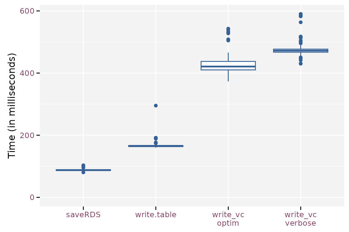
Boxplot of the write timings for the different methods.

Reading Data

mb <- microbenchmark(
  read.table = read.table(file.path(root, "base_R.tsv"), header = TRUE,
                          sep = "\t"),
  readRDS = readRDS(file.path(root, "base_R.rds")),
  read_vc.optim = read_vc("airbag_optimize", root),
  read_vc.verbose = read_vc("airbag_verbose", root)
)
mb$time <- mb$time / 1e6

The timings on reading the data is another story. Reading the binary format takes about 10% of the time needed to read the standard plain text format using read.table(). read_vc() takes about 214% (optimized) and 257% (verbose) of the time needed by read.table(), which at first seems strange because read_vc() calls read.table() to read the files and has some extra work to convert the variables to the correct data type. The main difference is that read_vc() knows the required data type a priori and passes this info to read.table(). Otherwise, read.table() has to guess the correct data type from the file.

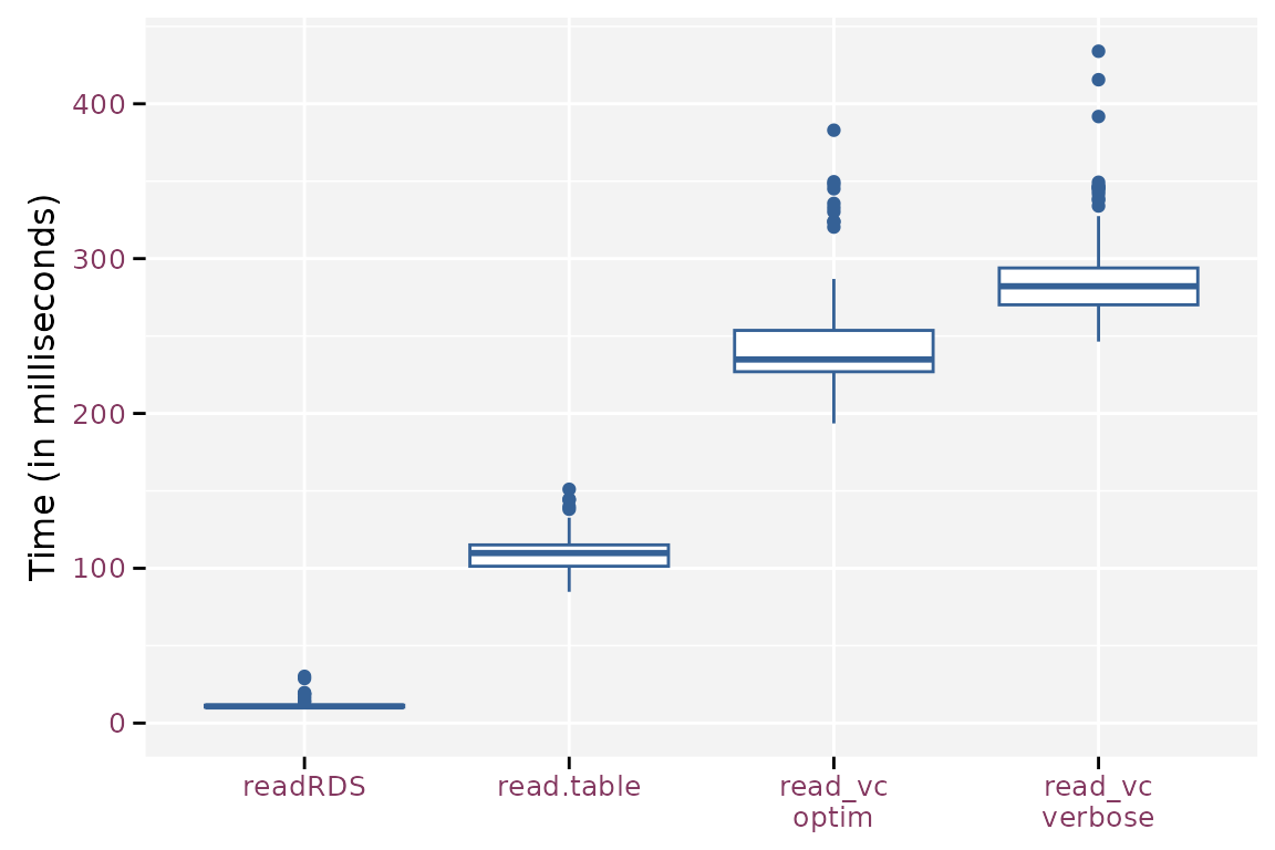
Boxplots for the read timings for the different methods.

Thierry Onkelinx