All the tests were done on an Arch Linux x86_64 machine with an Intel(R) Core(TM) i7 CPU (1.90GHz).
Empirical likelihood computation
We show the performance of computing empirical likelihood with
el_mean(). We test the computation speed with simulated
data sets in two different settings: 1) the number of observations
increases with the number of parameters fixed, and 2) the number of
parameters increases with the number of observations fixed.
Increasing the number of observations
We fix the number of parameters at
,
and simulate the parameter value and
matrices using rnorm(). In order to ensure convergence with
a large
,
we set a large threshold value using el_control().
library(ggplot2)
library(microbenchmark)
set.seed(3175775)
p <- 10
par <- rnorm(p, sd = 0.1)
ctrl <- el_control(th = 1e+10)
result <- microbenchmark(
  n1e2 = el_mean(matrix(rnorm(100 * p), ncol = p), par = par, control = ctrl),
  n1e3 = el_mean(matrix(rnorm(1000 * p), ncol = p), par = par, control = ctrl),
  n1e4 = el_mean(matrix(rnorm(10000 * p), ncol = p), par = par, control = ctrl),
  n1e5 = el_mean(matrix(rnorm(100000 * p), ncol = p), par = par, control = ctrl)
)
Below are the results:
result
#> Unit: microseconds
#>  expr        min          lq        mean      median          uq        max
#>  n1e2    421.418    465.5035    504.3654    484.6575    538.5125    640.544
#>  n1e3   1222.130   1442.4345   1563.9380   1533.6345   1672.5115   2536.609
#>  n1e4  11431.118  13188.2255  15421.7516  15792.7255  16956.6895  21539.877
#>  n1e5 180797.522 214986.9715 247646.9078 240679.9500 269075.2685 400521.431
#>  neval cld
#>    100 a
#>    100 a
#>    100  b
#>    100   c
autoplot(result)
#> Warning: `aes_string()` was deprecated in ggplot2 3.0.0.
#> ℹ Please use tidy evaluation idioms with `aes()`.
#> ℹ See also `vignette("ggplot2-in-packages")` for more information.
#> ℹ The deprecated feature was likely used in the microbenchmark package.
#>   Please report the issue at
#>   <https://github.com/joshuaulrich/microbenchmark/issues/>.
#> This warning is displayed once per session.
#> Call `lifecycle::last_lifecycle_warnings()` to see where this warning was
#> generated.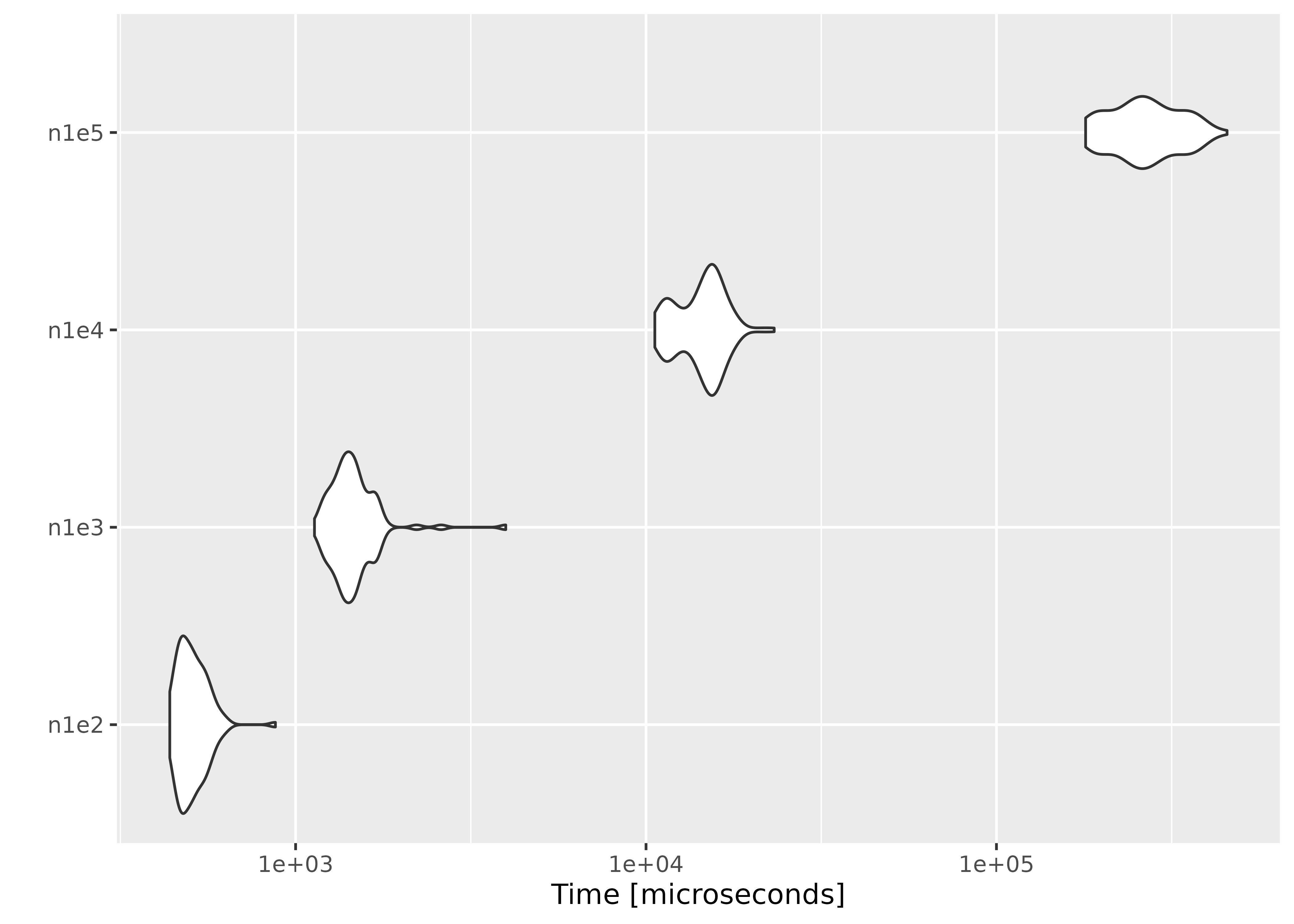
Increasing the number of parameters
This time we fix the number of observations at , and evaluate empirical likelihood at zero vectors of different sizes.
n <- 1000
result2 <- microbenchmark(
  p5 = el_mean(matrix(rnorm(n * 5), ncol = 5),
    par = rep(0, 5),
    control = ctrl
  ),
  p25 = el_mean(matrix(rnorm(n * 25), ncol = 25),
    par = rep(0, 25),
    control = ctrl
  ),
  p100 = el_mean(matrix(rnorm(n * 100), ncol = 100),
    par = rep(0, 100),
    control = ctrl
  ),
  p400 = el_mean(matrix(rnorm(n * 400), ncol = 400),
    par = rep(0, 400),
    control = ctrl
  )
)
result2
#> Unit: microseconds
#>  expr        min          lq       mean     median         uq        max neval
#>    p5    716.046    776.0715    849.110    800.918    861.674   4182.200   100
#>   p25   2939.549   2977.7750   3083.138   3016.488   3082.990   6469.468   100
#>  p100  23167.752  25958.2735  28305.902  26252.527  31401.517  48579.976   100
#>  p400 256622.755 281754.7815 319414.160 305358.553 344740.542 461553.556   100
#>  cld
#>  a
#>  a
#>   b
#>    c
autoplot(result2)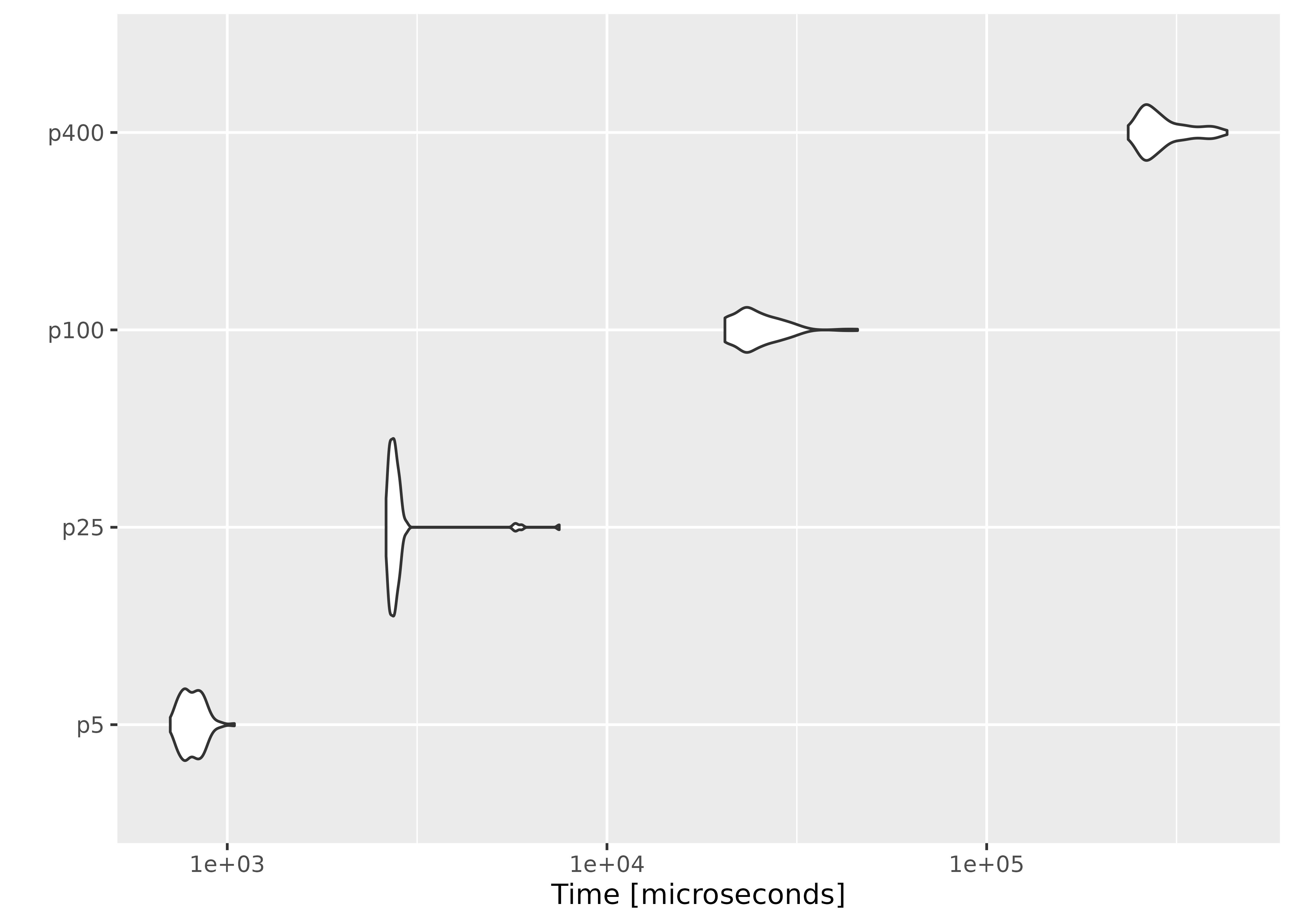
On average, evaluating empirical likelihood with a 100000×10 or 1000×400 matrix at a parameter value satisfying the convex hull constraint takes less than a second.