Overview
melt provides a unified framework for data analysis with empirical likelihood methods. A collection of functions is available to perform multiple empirical likelihood tests and construct confidence intervals for various models in ‘R’. melt offers an easy-to-use interface and flexibility in specifying hypotheses and calibration methods, extending the framework to simultaneous inferences. The core computational routines are implemented with the ‘Eigen’ ‘C++’ library and ‘RcppEigen’ interface, with ‘OpenMP’ for parallel computation. Details of the testing procedures are provided in Kim, MacEachern, and Peruggia (2023). The package has a companion paper by Kim, MacEachern, and Peruggia (2024). This work was supported by the U.S. National Science Foundation under Grants No. SES-1921523 and DMS-2015552.
Installation
You can install the latest stable release of melt from CRAN.
install.packages("melt")You can install the development version of melt from GitHub or R-universe.
# install.packages("pak")
pak::pak("ropensci/melt")
install.packages("melt", repos = "https://ropensci.r-universe.dev")Main functions
melt provides an intuitive API for performing the most common data analysis tasks:
-
el_mean()computes empirical likelihood for the mean. -
el_lm()fits a linear model with empirical likelihood. -
el_glm()fits a generalized linear model with empirical likelihood. -
confint()computes confidence intervals for model parameters. -
confreg()computes confidence region for model parameters. -
elt()tests a hypothesis with various calibration options. -
elmt()performs multiple testing simultaneously.
Usage
library(melt)
set.seed(971112)

## Test for the mean
data("precip")
(fit <- el_mean(precip, par = 30))
#>
#>  Empirical Likelihood
#>
#> Model: mean
#>
#> Maximum EL estimates:
#> [1] 34.89
#>
#> Chisq: 8.285, df: 1, Pr(>Chisq): 0.003998
#> EL evaluation: converged


## Adjusted empirical likelihood calibration
elt(fit, rhs = 30, calibrate = "ael")
#>
#>  Empirical Likelihood Test
#>
#> Hypothesis:
#> par = 30
#>
#> Significance level: 0.05, Calibration: Adjusted EL
#>
#> Statistic: 7.744, Critical value: 3.841
#> p-value: 0.005389
#> EL evaluation: converged


## Bootstrap calibration
elt(fit, rhs = 30, calibrate = "boot")
#>
#>  Empirical Likelihood Test
#>
#> Hypothesis:
#> par = 30
#>
#> Significance level: 0.05, Calibration: Bootstrap
#>
#> Statistic: 8.285, Critical value: 3.84
#> p-value: 0.0041
#> EL evaluation: converged


## F calibration
elt(fit, rhs = 30, calibrate = "f")
#>
#>  Empirical Likelihood Test
#>
#> Hypothesis:
#> par = 30
#>
#> Significance level: 0.05, Calibration: F
#>
#> Statistic: 8.285, Critical value: 3.98
#> p-value: 0.005318
#> EL evaluation: converged


## Linear model
data("mtcars")
fit_lm <- el_lm(mpg ~ disp + hp + wt + qsec, data = mtcars)
summary(fit_lm)
#>
#>  Empirical Likelihood
#>
#> Model: lm
#>
#> Call:
#> el_lm(formula = mpg ~ disp + hp + wt + qsec, data = mtcars)
#>
#> Number of observations: 32
#> Number of parameters: 5
#>
#> Parameter values under the null hypothesis:
#> (Intercept)        disp          hp          wt        qsec
#>       29.04        0.00        0.00        0.00        0.00
#>
#> Lagrange multipliers:
#> [1] -260.167   -2.365    1.324  -59.781   25.175
#>
#> Maximum EL estimates:
#> (Intercept)        disp          hp          wt        qsec
#>   27.329638    0.002666   -0.018666   -4.609123    0.544160
#>
#> logL: -327.6 , logLR: -216.7
#> Chisq: 433.4, df: 4, Pr(>Chisq): < 2.2e-16
#> Constrained EL: converged
#>
#> Coefficients:
#>              Estimate   Chisq Pr(>Chisq)
#> (Intercept) 27.329638 443.208    < 2e-16 ***
#> disp         0.002666   0.365    0.54575
#> hp          -0.018666  10.730    0.00105 **
#> wt          -4.609123 439.232    < 2e-16 ***
#> qsec         0.544160 440.583    < 2e-16 ***
#> ---
#> Signif. codes:  0 '***' 0.001 '**' 0.01 '*' 0.05 '.' 0.1 ' ' 1
cr <- confreg(fit_lm, parm = c("disp", "hp"), npoints = 200)
plot(cr)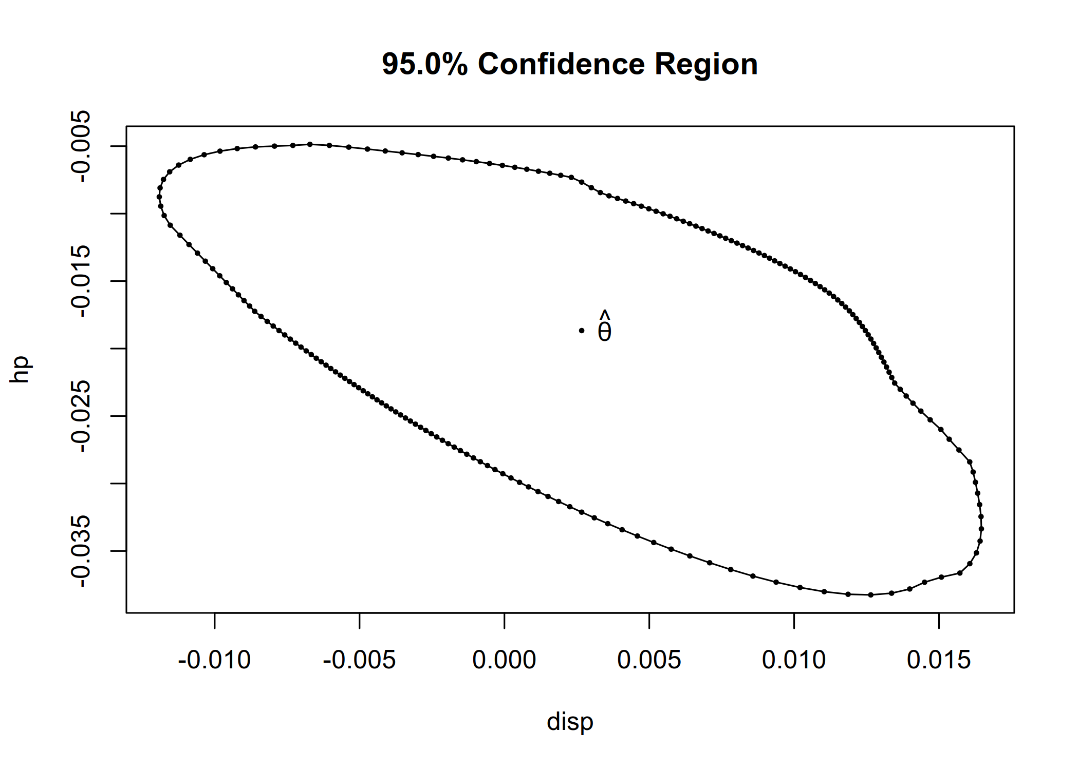
data("clothianidin")
fit2_lm <- el_lm(clo ~ -1 + trt, data = clothianidin)
summary(fit2_lm)
#>
#>  Empirical Likelihood
#>
#> Model: lm
#>
#> Call:
#> el_lm(formula = clo ~ -1 + trt, data = clothianidin)
#>
#> Number of observations: 102
#> Number of parameters: 4
#>
#> Parameter values under the null hypothesis:
#>     trtNaked trtFungicide       trtLow      trtHigh
#>            0            0            0            0
#>
#> Lagrange multipliers:
#> [1] -4.116e+06 -7.329e-01 -1.751e+00 -1.418e-01
#>
#> Maximum EL estimates:
#>     trtNaked trtFungicide       trtLow      trtHigh
#>       -4.479       -3.427       -2.800       -1.307
#>
#> logL: -918.9 , logLR: -447.2
#> Chisq: 894.4, df: 4, Pr(>Chisq): < 2.2e-16
#> EL evaluation: maximum iterations reached
#>
#> Coefficients:
#>              Estimate   Chisq Pr(>Chisq)
#> trtNaked       -4.479 411.072    < 2e-16 ***
#> trtFungicide   -3.427  59.486   1.23e-14 ***
#> trtLow         -2.800  62.955   2.11e-15 ***
#> trtHigh        -1.307   4.653      0.031 *
#> ---
#> Signif. codes:  0 '***' 0.001 '**' 0.01 '*' 0.05 '.' 0.1 ' ' 1
confint(fit2_lm)
#>                  lower      upper
#> trtNaked     -5.002118 -3.9198229
#> trtFungicide -4.109816 -2.6069870
#> trtLow       -3.681837 -1.9031795
#> trtHigh      -2.499165 -0.1157222


## Generalized linear model
data("thiamethoxam")
fit_glm <- el_glm(visit ~ log(mass) + fruit + foliage + var + trt,
  family = quasipoisson(link = "log"), data = thiamethoxam,
  control = el_control(maxit = 100, tol = 1e-08, nthreads = 4)
)
summary(fit_glm)
#>
#>  Empirical Likelihood
#>
#> Model: glm (quasipoisson family with log link)
#>
#> Call:
#> el_glm(formula = visit ~ log(mass) + fruit + foliage + var +
#>     trt, family = quasipoisson(link = "log"), data = thiamethoxam,
#>     control = el_control(maxit = 100, tol = 1e-08, nthreads = 4))
#>
#> Number of observations: 165
#> Number of parameters: 8
#>
#> Parameter values under the null hypothesis:
#> (Intercept)   log(mass)       fruit     foliage       varGZ    trtSpray
#>     -0.1098      0.0000      0.0000      0.0000      0.0000      0.0000
#>   trtFurrow     trtSeed         phi
#>      0.0000      0.0000      1.4623
#>
#> Lagrange multipliers:
#> [1]   1319.19    210.54    -12.99 -24069.07   -318.90   -189.14    -53.35
#> [8]    262.32   -170.21
#>
#> Maximum EL estimates:
#> (Intercept)   log(mass)       fruit     foliage       varGZ    trtSpray
#>    -0.10977     0.24750     0.04654   -19.40632    -0.25760     0.06724
#>   trtFurrow     trtSeed
#>    -0.03634     0.34790
#>
#> logL: -2272 , logLR: -1429
#> Chisq: 2859, df: 7, Pr(>Chisq): < 2.2e-16
#> Constrained EL: initialization failed
#>
#> Coefficients:
#>              Estimate   Chisq Pr(>Chisq)
#> (Intercept)  -0.10977   0.090      0.764
#> log(mass)     0.24750 425.859    < 2e-16 ***
#> fruit         0.04654  29.024   7.15e-08 ***
#> foliage     -19.40632  65.181   6.83e-16 ***
#> varGZ        -0.25760  17.308   3.18e-05 ***
#> trtSpray      0.06724   0.860      0.354
#> trtFurrow    -0.03634   0.217      0.641
#> trtSeed       0.34790  19.271   1.13e-05 ***
#> ---
#> Signif. codes:  0 '***' 0.001 '**' 0.01 '*' 0.05 '.' 0.1 ' ' 1
#>
#> Dispersion for quasipoisson family: 1.462288


## Test of no treatment effect
contrast <- c(
  "trtNaked - trtFungicide", "trtFungicide - trtLow", "trtLow - trtHigh"
)
elt(fit2_lm, lhs = contrast)
#>
#>  Empirical Likelihood Test
#>
#> Hypothesis:
#> trtNaked - trtFungicide = 0
#> trtFungicide - trtLow = 0
#> trtLow - trtHigh = 0
#>
#> Significance level: 0.05, Calibration: Chi-square
#>
#> Statistic: 26.6, Critical value: 7.815
#> p-value: 7.148e-06
#> Constrained EL: converged


## Multiple testing
contrast2 <- rbind(
  c(0, 0, 0, 0, 0, 1, 0, 0),
  c(0, 0, 0, 0, 0, 0, 1, 0),
  c(0, 0, 0, 0, 0, 0, 0, 1)
)
elmt(fit_glm, lhs = contrast2)
#>
#>  Empirical Likelihood Multiple Tests
#>
#> Overall significance level: 0.05
#>
#> Calibration: Multivariate chi-square
#>
#> Hypotheses:
#>               Estimate  Chisq Df
#> trtSpray = 0   0.06724  0.860  1
#> trtFurrow = 0 -0.03634  0.217  1
#> trtSeed = 0    0.34790 19.271  1
Please note that this package is released with a Contributor Code of Conduct. By contributing to this project, you agree to abide by its terms.