How to Compute Historical Rates from B3 Future Prices

Introduction

The template b3-futures-settlement-prices allows you to fetch historical settlement prices for future contracts from B3 (Brasil, Bolsa, Balcão), the Brazilian stock exchange and derivatives market. This vignette provides a step-by-step guide on how to retrieve, process, and analyze this data using the rb3 package.

The futures contract settlement prices are published daily by B3. These settlement prices represent the official daily closing values used for marking positions to market and calculating margin requirements.

The data is publicly available on the B3 website through their Trading session settlements page. This page provides one of the longest available historical records of futures contract prices. We’ll use this historical pricing data to analyze trends, term structures, and other patterns in Brazilian futures markets.

library(rb3) # B3 data access
library(ggplot2) # data visualization
library(stringr) # string manipulation
library(dplyr) # data transformation
library(bizdays) # business days calculations

Fetching historical data

To analyze historical futures data, we’ll collect settlement prices at regular intervals. We’ll fetch data for the first Monday of each week over a two-year period (2021-2022).

First, we generate a sequence of dates representing first Mondays from January 2021 through December 2022. We then adjust these dates using the following() function from the bizdays package to ensure we only get valid trading days on the B3 calendar. We use “first mon” to select Mondays and a 7-day interval for weekly samples. This provides regular sampling points while keeping the dataset manageable.

After selecting our dates, we use the fetch_marketdata() function from the rb3 package to:

Download the futures settlement prices data from B3’s website
Parse the raw data into a structured format
Store it in the rb3 package’s internal database for efficient queries

This process avoids repeated downloads and provides consistent access to the data. The stored data creates the dataset b3-futures-settlement-prices, which can be queried and analyzed efficiently.

dates <- getdate("first mon", seq(as.Date("2021-01-01"), as.Date("2022-12-24"), by = 7), "actual") |>
  following("Brazil/B3")
fetch_marketdata("b3-futures-settlement-prices", refdate = dates)

By leveraging the rb3 and bizdays packages together, we can efficiently manage and analyze historical market data from B3, enabling us to explore various aspects of the Brazilian financial markets.

Querying the data

After fetching the historical futures data, we can query it using the futures_get() function from the rb3 package. This function allows us to retrieve the data stored in the internal database efficiently. Note that futures_get() uses lazy evaluation, meaning it only loads the data when explicitly requested.

# Retrieve the futures settlement prices data
df <- futures_get() |>
  collect()

Call the futures_get() function to retrieve the dataset. Then, use the collect() function to load the data into a data frame for further analysis.

# Display the first few rows of the dataset
head(df)
#> # A tibble: 6 × 8
#>   refdate    symbol commodity maturity_code previous_price  price price_change
#>   <date>     <chr>  <chr>     <chr>                  <dbl>  <dbl>        <dbl>
#> 1 2021-01-04 AFSF21 AFS       F21                   14605  14605           0  
#> 2 2021-01-04 AFSG21 AFS       G21                   14670. 14747          76.7
#> 3 2021-01-04 AFSH21 AFS       H21                   14718. 14792.         74.8
#> 4 2021-01-04 AFSJ21 AFS       J21                   14783. 14853.         70.2
#> 5 2021-01-04 AFSK21 AFS       K21                   14831. 14903.         71.5
#> 6 2021-01-04 AFSM21 AFS       M21                   14880. 14953.         73.2
#> # ℹ 1 more variable: settlement_value <dbl>

In this example, we see how to use the function futures_get() to access the data stored in the b3-futures-settlement-prices dataset.

This queried data can now be used for further analysis, such as calculating historical nominal and real interest rates, implied inflation, and forward rates.

Historical nominal interest rates

Interest rates can be derived from the prices of futures contracts. DI1 contracts mature on the first day of the month. The code below generates the maturity dates from the three characters of the maturity code. Then, we calculate the implied rates considering that the notional value of the contracts is 100000.

$\text{Adjusted Rate} = \left(\frac{100000}{\text{Price}}\right)^{\frac{252}{\text{Business Days}}} - 1$

di1_futures <- df |>
  filter(commodity == "DI1") |>
  mutate(
    maturity_date = maturity2date(maturity_code),
    fixing = following(maturity_date, "Brazil/ANBIMA"),
    business_days = bizdays(refdate, maturity_date, "Brazil/ANBIMA"),
    adjusted_tax = (100000 / price)^(252 / business_days) - 1
  ) |>
  filter(business_days > 0)

In the graph below we see the dynamics of the nominal interest rates of the contracts DI1F23 and DI1F33. These contracts are exactly 10 years distant from each other.

di1_futures |>
  filter(symbol %in% c("DI1F23", "DI1F33")) |>
  ggplot(aes(x = refdate, y = adjusted_tax, color = symbol, group = symbol)) +
  geom_line() +
  labs(
    title = "DI1 Future Rates - Nominal Interest Rates",
    caption = "Source B3 - package rb3",
    x = "Date",
    y = "Interest Rates",
    color = "Symbol"
  ) +
  scale_y_continuous(labels = scales::percent)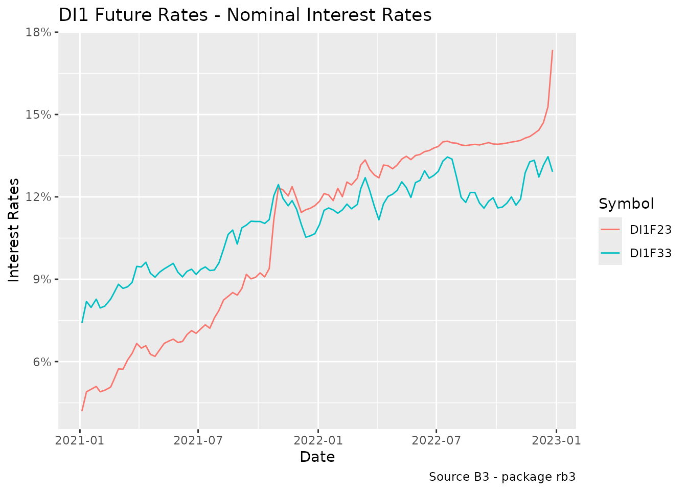

DI1 Future Rates - Nominal Interest Rates

Historical real interest rates

Differently from DI1 contracts, that trade nominal interest rates, the DAP contracts trade real interest rates. DAP contracts matures on the 15th day of the month. The code below generates the maturity dates from the three characters of the maturity code. Then, we calculate the implied rates considering that the notional value of the contracts is 100000, exactly as we did for the DI1 contracts.

dap_futures <- df |>
  filter(commodity == "DAP") |>
  mutate(
    maturity_date = maturity2date(maturity_code, "15th day"),
    fixing = following(maturity_date, "Brazil/ANBIMA"),
    business_days = bizdays(refdate, maturity_date, "Brazil/ANBIMA"),
    adjusted_tax = (100000 / price)^(252 / business_days) - 1
  ) |>
  filter(business_days > 0)

The graphic below shows the dynamics of the real interest rates of the contracts DAPF23 and DAPK35. These contracts are exactly 12 years distant from each other. Since we don’t have a 10-year contract, we use the 12-year contract as a reference to observe the dynamics of short and long term real interest rates.

dap_futures |>
  filter(symbol %in% c("DAPF23", "DAPK35")) |>
  ggplot(aes(x = refdate, y = adjusted_tax, group = symbol, color = symbol)) +
  geom_line() +
  geom_point() +
  labs(
    title = "DAP Future Rates - Real Interest Rates",
    caption = "Source B3 - package rb3",
    x = "Date",
    y = "Interest Rates",
    color = "Symbol"
  ) +
  scale_y_continuous(labels = scales::percent)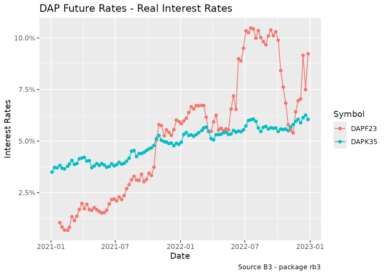

DAP Future Rates - Real Interest Rates

Implied inflation

By comparing the real and nominal interest rates, we can derive the forward inflation implied in these contracts. Specifically, we use the DI1F23 and DAPF23 contracts, which mature in the same month with only a few days’ difference. The implied inflation can be calculated by dividing the prices of these contracts.

$\text{Inflation} \approx \frac{\text{DAPF23}}{\text{DI1F23}} - 1$

infl_futures <- df |>
  filter(symbol %in% c("DI1F23", "DAPF23"))

infl_expec <- infl_futures |>
  select(symbol, price, refdate) |>
  tidyr::pivot_wider(names_from = symbol, values_from = price) |>
  mutate(inflation = DAPF23 / DI1F23 - 1)

infl_expec |>
  ggplot(aes(x = refdate, y = inflation)) +
  geom_line() +
  geom_point() +
  labs(
    x = "Date", y = "Inflation",
    title = "Implied Inflation from futures DI1F23, DAPF23",
    caption = "Source B3 - package rb3"
  )

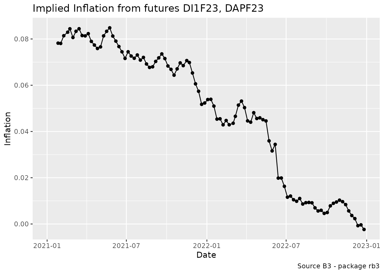
Implied Inflation from futures

We can observe that, as the contracts approach maturity, the implied inflation converges to zero, as expected. To overcome this bias, let’s redo the graph for the F24 maturity.

df |>
  filter(symbol %in% c("DI1F24", "DAPF24")) |>
  select(symbol, price, refdate) |>
  tidyr::pivot_wider(names_from = symbol, values_from = price) |>
  mutate(inflation = DAPF24 / DI1F24 - 1) |>
  na.omit() |>
  ggplot(aes(x = refdate, y = inflation)) +
  geom_line() +
  geom_point() +
  labs(
    x = "Date", y = "Inflation",
    title = "Implied Inflation from futures DI1F24, DAPF24",
    caption = "Source B3 - package rb3"
  )

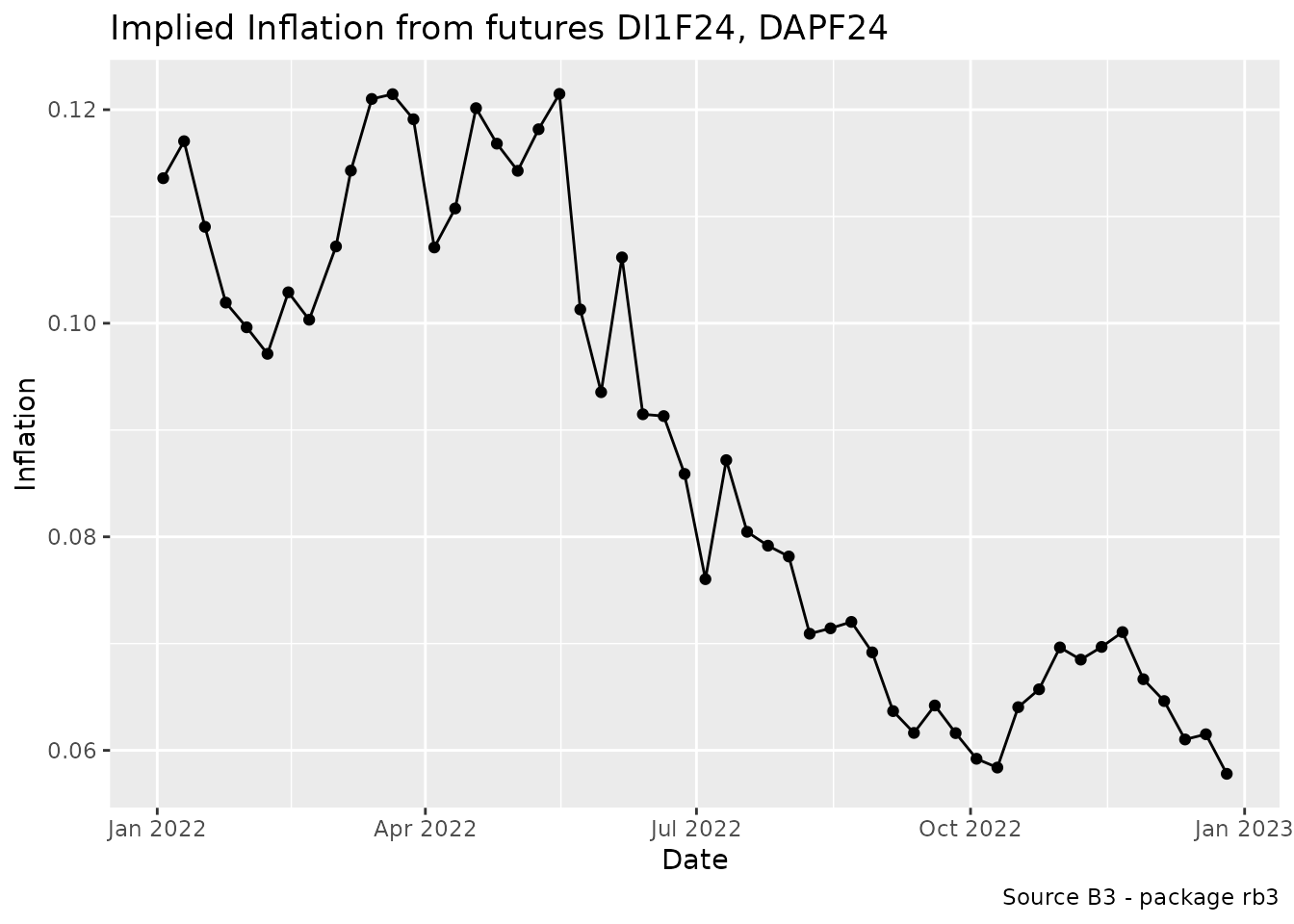
Implied Inflation from futures

Forward rates

The 10-year forward rates implied in DI1 futures prices can be computed using the DI1F23 and DI1F33 contracts. These contracts are used to calculate the 10-year forward rates, which range from January 2023 to January 2033.

Here it follows the steps to calculate the forward rates.

Filter Data: filter the dataframe df to include only rows where the symbol is either “DI1F23” or “DI1F33”. Save this filtered dataframe in a new dataframe called df_fut.

df_fut <- df |>
  filter(symbol %in% c("DI1F23", "DI1F33"))

Calculate Maturity Date and Business Days: convert the maturity_code to maturity_date and adjust it to the next business day according to the “Brazil/ANBIMA” calendar. Calculate the number of business days between the reference date (refdate) and the maturity date.

df_fut <- df_fut |>
  mutate(
    maturity_date = maturity2date(maturity_code) |>
      following("Brazil/ANBIMA"),
    business_days = bizdays(refdate, maturity_date, "Brazil/ANBIMA")
  )

Calculate the Difference in Business Days: calculate the difference in business days between the DI1F23 and DI1F33 contracts. Save this information in a new dataframe called df_du.

df_du <- df_fut |>
  select(refdate, symbol, business_days) |>
  tidyr::pivot_wider(names_from = symbol, values_from = business_days) |>
  mutate(
    du = DI1F33 - DI1F23
  ) |>
  select(refdate, du)

Join Dataframes: join the df_fut and df_du dataframes by the refdate column. Select only the refdate, symbol, and price columns from the df_fut dataframe. Pivot the df_fut dataframe to have the symbol as columns and the price as values. Now we have the prices of the futures and the business days between them, for each date, in the same row.

df_fut <- df_fut |>
  select(refdate, symbol, price) |>
  tidyr::pivot_wider(names_from = symbol, values_from = price) |>
  inner_join(df_du, by = "refdate")

Calculate the Forward Rates: calculate the 10-year forward rates using the formula below.

$\text{Forward Rate} = \left(\frac{\text{DI1F23}}{\text{DI1F33}}\right)^{\frac{252}{\text{Business Days}}} - 1$

df_fwd <- df_fut |>
  mutate(
    fwd = (DI1F23 / DI1F33)^(252 / du) - 1
  ) |>
  select(refdate, fwd) |>
  na.omit()

Make a graph showing the dynamics of the 10-year forward rates from January 2023 to January 2033.

df_fwd |>
  ggplot(aes(x = refdate, y = fwd)) +
  geom_line() +
  labs(
    x = "Date", y = "Forward Rates",
    title = "Historical 10Y Forward Rates - F23:F33",
    caption = "Source B3 - package rb3"
  )

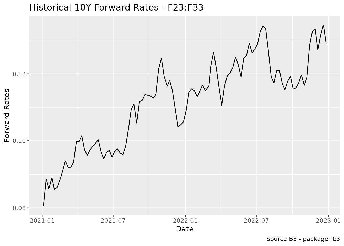
Forward Rates

Conclusion

In this document, we demonstrated how to fetch and analyze historical futures contract settlement prices from B3 (Brasil, Bolsa, Balcão). By leveraging the rb3 package, we were able to efficiently download, query, and process the data to derive meaningful insights.

We covered the following key steps:

Fetching Historical Data: We collected settlement prices at regular intervals over a two-year period and stored them in the rb3 package’s internal database.
Querying the Data: Using the futures_get() function, we retrieved the data for further analysis.
Calculating Historical Nominal and Real Interest Rates: We derived interest rates from the prices of DI1 and DAP futures contracts.
Implied Inflation: By comparing the real and nominal interest rates, we calculated the forward inflation implied in the contracts.
Forward Rates: We computed the 10-year forward rates using the DI1F23 and DI1F33 contracts.

Through these analyses, we gained insights into the trends, term structures, and other patterns in Brazilian futures markets. The ability to efficiently process and analyze this data is crucial for market participants, researchers, and policymakers to make informed decisions.

By following the steps outlined in this document, you can replicate the analysis and adapt it to your specific needs. The rb3 package provides a powerful toolset for accessing and analyzing B3 market data, enabling you to explore various aspects of the Brazilian financial markets.