Fetching B3 Yield Curves

Introduction

The template b3-reference-rates allows you to fetch historical yield curves from B3, the Brazilian stock exchange. This vignette provides a step-by-step guide on how to retrieve and visualize these curves using the rb3 package.

The yield curve is a key tool in financial markets, offering insights into interest rate expectations, inflation outlook, and economic sentiment. In Brazil, the local exchange (B3) publishes a set of reference yield curves built from the pricing of interest rate futures contracts. B3 provides historical yield curves on its website. These curves are built using interest rate futures contracts.

This vignette demonstrates how to retrieve and analyze historical yield curves from B3 using the rb3 R package. We focus on three main curves:

PRE: nominal interest rate curve, derived from fixed-rate (DI) futures.
DIC: real interest rate curve, based on IPCA-indexed futures (Cupom de IPCA).
DOC: FX-linked curve (Cupom Cambial), reflecting the interest rate differential between BRL and USD.

For further details on how B3 constructs these curves, see B3’s reference rate documentation (PDF).

library(rb3)
library(ggplot2)
library(dplyr)
library(bizdays)

Fetching the data

In this section, we will fetch the historical yield curve data for the years 2021 to 2025. The yield curves are constructed using interest rate futures data, which is provided by B3. To obtain the data, we follow these two main steps:

Selecting Reference Dates

We begin by selecting the first business day of each year between 2021 and 2025 using the getdate() function. This provides a set of consistent reference points, free from seasonal distortions or holiday effects, which are ideal for comparing yield curves over time.

2. Fetching and Storing Market Data

The fetch_marketdata() function is used to download the yield curve data for the selected reference dates using the template b3-reference-rates. This template is designed to fetch the reference rates from B3’s systems. This function fetches data directly from B3’s systems and stores it in a structured format within the rb3 package database. The data is stored locally in an optimized structure, allowing for efficient querying and analysis in subsequent steps.

We specify the curve_name argument to request data for three different yield curves:

PRE: The Nominal Interest Rate curve. This curve represents the market’s expectations for accumulated interbank interest rates (DI - interbank deposit) from the reference date to each forward date. It is constructed from DI1 interest futures and reflects the nominal yield investors require, inclusive of inflation expectations and real interest.
DOC: The Cupom Cambial (FX Swap Implied Rate) curve. This curve reflects the interest rate differential between Brazilian real (BRL) and U.S. dollar (USD), as implied by FX swap contracts. It is derived from contracts where the local leg pays fixed BRL interest and the foreign leg pays USD, adjusted by the spot and forward exchange rate. This curve is useful for pricing instruments that involve currency exposure or hedging strategies.
DIC: The IPCA-Linked (Real Interest Rate) curve, also referred to as the Cupom de IPCA. This curve represents the real interest rate (excluding inflation) implied by futures contracts indexed to the Brazilian consumer price index (IPCA). It is used to assess the market’s expectation of real returns and is essential for pricing inflation-linked bonds (like NTN-B).

The curve_name argument allows us to specify which of these three curves we want data for. By passing a vector like c("DIC", "DOC", "PRE"), we are telling the function to retrieve data for all three curves for the selected reference dates.

dates <- getdate("first bizday", 2021:2025, "Brazil/B3")
fetch_marketdata("b3-reference-rates", refdate = dates, curve_name = c("DIC", "DOC", "PRE"))

After the data is stored, it becomes available for querying through the following functions:

yc_brl_get(): This function retrieves the Brazilian nominal yield curve data (PRE curve), which includes accumulated interbank interest rates (DI) for the selected dates.
yc_usd_get(): This function retrieves the FX-linked yield curve data (DOC curve), reflecting the interest rate differential between Brazilian real (BRL) and U.S. dollar (USD).
yc_ipca_get(): This function retrieves the Brazilian real interest rate curve (DIC curve), which is based on futures contracts linked to the Brazilian Consumer Price Index (IPCA).

PRE Curve (DI rates)

In this section, we will visualize the yield curves for Nominal Interest Rate, based on the previously fetched data.

This section focuses on the PRE curve, which represents the nominal interest rate curve built using DI1 futures contracts. These contracts reflect the market’s expectations for the cumulative interbank interest rates (DI rates) from the reference date to each future maturity.

The PRE curve is essential for understanding nominal yield dynamics in Brazil’s fixed income market, and it’s commonly used for pricing public and private debt instruments.

df_yc_brl <- yc_brl_get() |>
  filter(forward_date < "2035-01-01") |>
  collect()

We apply a filter to restrict the forward dates to maturities before January 1st, 2035. This is because after this point, the futures market becomes significantly less liquid, and the yield curve relies more heavily on extrapolation methods rather than observable market data. Including such long maturities could introduce distortions or give a false sense of precision beyond what the market actually supports.

p <- ggplot(
  df_yc_brl,
  aes(
    x = forward_date,
    y = r_252,
    group = refdate,
    color = factor(refdate)
  )
) +
  geom_line(linewidth = 1) +
  labs(
    title = "Yield Curves for Brazil",
    subtitle = "Built using interest rates future contracts",
    caption = "Source B3 - package rb3",
    x = "Forward Date",
    y = "Annual Interest Rate",
    color = "Reference Date"
  ) +
  theme_light() +
  scale_y_continuous(labels = scales::percent)

print(p)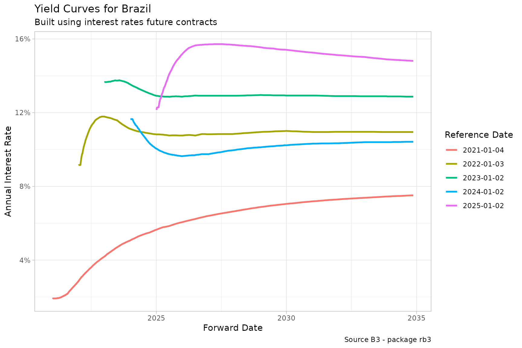

Yield Curves for Brazil

This plot shows how the nominal yield curve evolves over time, with different lines representing the curves on each reference date (first business day of each year from 2021 to 2025). You can observe shifts in market expectations for interest rates and detect periods of steepening, flattening, or inversion of the curve, which often signal changes in monetary policy outlook or economic sentiment.

IPCA Curve (DIC curve)

This section analyzes the DIC curve, which represents the real interest rate implied by futures contracts indexed to the Brazilian consumer price index (IPCA). It reflects market expectations for inflation-adjusted (real) returns.

The DIC curve is especially relevant for pricing inflation-linked bonds (such as NTN-Bs) and for analyzing the market’s perception of long-term inflation dynamics.

df_yc_ipca <- yc_ipca_get() |>
  collect()

p <- ggplot(
  df_yc_ipca |> filter(biz_days > 21, biz_days < 1008),
  aes(
    x = forward_date,
    y = r_252,
    group = refdate,
    color = factor(refdate)
  )
) +
  geom_line(linewidth = 1) +
  labs(
    title = "DIxIPCA Yield Curves for Brazil",
    subtitle = "Built using interest rates future contracts",
    caption = "Source B3 - package rb3",
    x = "Forward Date",
    y = "Annual Interest Rate",
    color = "Reference Date"
  ) +
  theme_light() +
  scale_y_continuous(labels = scales::percent)

print(p)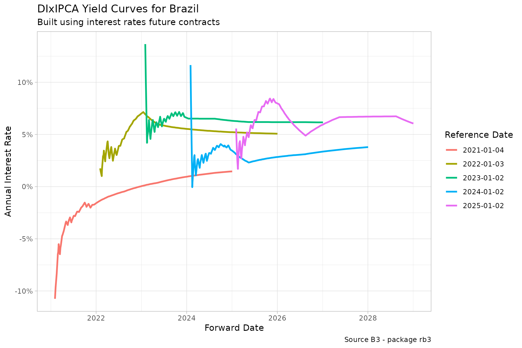

DIxIPCA Yield Curves for Brazil

This plot illustrates how real interest rates have evolved across different reference dates. These rates reflect the market’s view on long-term monetary stability and inflation control.

Cupom Limpo (USD - DOC curve)

This section focuses on the DOC curve, which represents the cupom cambial — the interest rate differential between the Brazilian real (BRL) and the U.S. dollar (USD), derived from FX swap contracts.

The DOC curve is constructed using the pricing of contracts where one leg pays fixed BRL interest and the other is tied to the USD. It reflects market expectations for exchange rate and interest rate spreads.

df_yc_usd <- yc_usd_get() |>
  filter(forward_date < "2035-01-01") |>
  collect()

As with other curves, we filter out maturities beyond 2035. This is because FX futures contracts tend to be illiquid at longer horizons, and extrapolated values beyond that point may not reflect reliable market pricing.

p <- ggplot(
  df_yc_usd |> filter(biz_days > 21, biz_days < 2520),
  aes(
    x = forward_date,
    y = r_360,
    group = refdate,
    color = factor(refdate)
  )
) +
  geom_line(linewidth = 1) +
  labs(
    title = "Cupom Limpo (USD) Yield Curves for Brazil",
    subtitle = "Built using interest rates future contracts",
    caption = "Source B3 - package rb3",
    x = "Forward Date",
    y = "Annual Interest Rate",
    color = "Reference Date"
  ) +
  theme_light() +
  scale_y_continuous(labels = scales::percent)

print(p)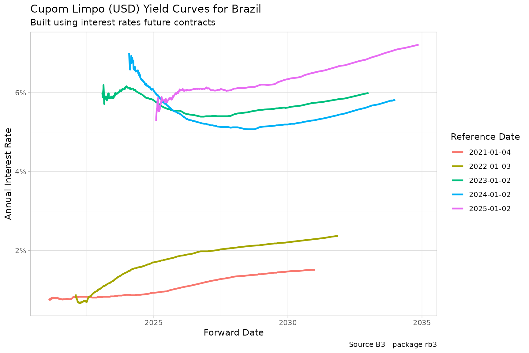

Cupom Limpo (USD) Yield Curves for Brazil

This curve provides insight into how the market prices currency risk and interest rate differentials between Brazil and the U.S., which are key for investors operating in cross-border markets or using hedging strategies.

Break-even Inflation: PRE vs DIC

By comparing the nominal yield curve (PRE) with the real yield curve (DIC), we can derive the implied inflation expectation priced by the market. This difference, known as break-even inflation, represents the inflation rate that would make an investor indifferent between holding nominal versus inflation-linked instruments.

The formula is straightforward:

$\text{Implied Inflation} = (1 + r_{\text{nominal}}) / (1 + r_{\text{real}}) - 1$

Where $r_{\text{nominal}}$ comes from the PRE curve and $r_{\text{real}}$ from the DIC curve. For simplicity, we use the approximation:

$\text{Implied Inflation} \approx r_{\text{nominal}} - r_{\text{real}}$

# Load and prepare PRE and DIC curves
pre <- df_yc_brl |>
  select(refdate, forward_date, r_nominal = r_252)

ipca <- df_yc_ipca |>
  select(refdate, forward_date, r_real = r_252)

# Join both curves by refdate and forward_date
df_be <- inner_join(pre, ipca, by = c("refdate", "forward_date")) |>
  mutate(break_even = r_nominal - r_real)

p <- ggplot(
  df_be,
  aes(
    x = forward_date,
    y = break_even,
    group = refdate,
    color = factor(refdate)
  )
) +
  geom_line(linewidth = 1) +
  labs(
    title = "Implied Inflation (Break-even) from Yield Curves",
    subtitle = "Calculated as PRE (nominal) minus DIC (real)",
    caption = "Source B3 - package rb3",
    x = "Forward Date",
    y = "Annual Implied Inflation Rate",
    color = "Reference Date"
  ) +
  theme_light() +
  scale_y_continuous(labels = scales::percent)

print(p)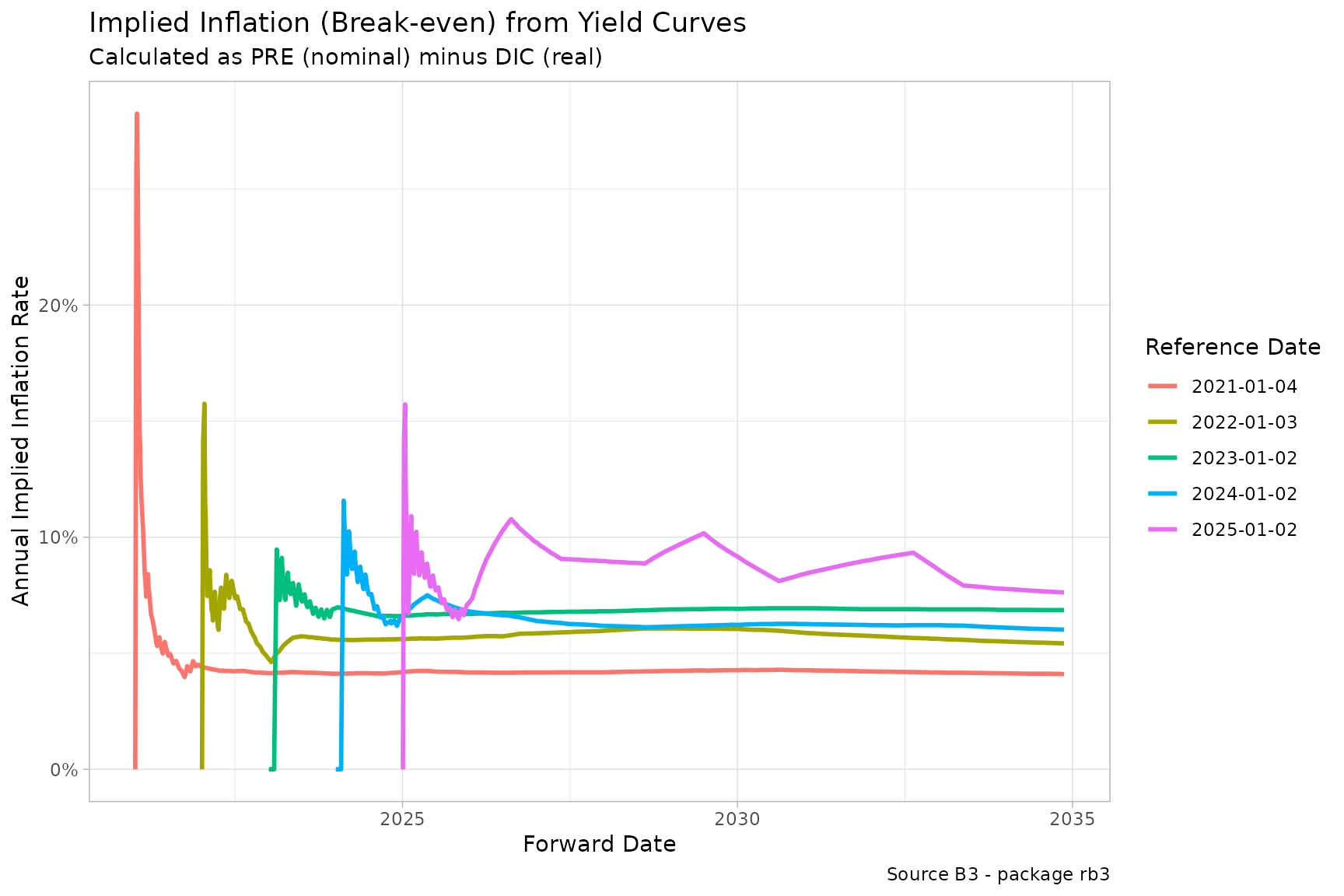

Break-even Inflation

This chart shows the inflation expectations embedded in the market at different points in time and across different maturities. Steeper break-even curves may indicate expected inflationary pressures ahead, while flatter curves may reflect confidence in inflation control or economic deceleration.

Such analysis is useful for:

Pricing inflation-linked bonds
Assessing central bank credibility
Supporting asset allocation decisions (e.g., real vs nominal fixed income)

Conclusion

In this vignette, we explored how to fetch and visualize historical yield curves from the Brazilian exchange (B3) using the rb3 package. We covered three types of curves:

PRE: nominal interest rates, built from fixed-rate futures contracts.
DIC: real interest rates (inflation-adjusted), derived from IPCA-indexed futures.
DOC: FX-linked rates (cupom cambial), representing BRL-USD interest differentials.

We also showed how to extract break-even inflation expectations by comparing the nominal and real curves — a powerful tool for understanding the market’s inflation outlook.

These curves are widely used in:

Monetary policy analysis
Fixed income pricing
Inflation forecasting
Asset allocation and risk management

The rb3 package provides a simple yet flexible interface for retrieving and working with this data directly in R.

As next steps, you might consider:

Tracking curve movements on a daily basis
Building yield curve interpolation models
Estimating forward rates or zero-coupon curves
Backtesting strategies based on curve dynamics

Feel free to explore the package documentation and source code for more advanced features and use cases.

Happy analyzing!