library(rnaturalearth)
library(sf)
#> Linking to GEOS 3.12.1, GDAL 3.8.5, PROJ 9.4.0; sf_use_s2() is TRUE
Available data
There are a lot of data that can be downloaded from Natural Earth with
ne_download(). These data are divided into two main
categories: physical and cultural vector data. The
df_layers_physical and df_layers_cultural data
frames included in the rnaturalearth packages show what
layer of data can be downloaded.
Physical vector data
data(df_layers_physical)

knitr::kable(
  df_layers_physical,
  caption = "physical vector data available via ne_download()"
)| layer | scale10 | scale50 | scale110 |
|---|---|---|---|
| antarctic_ice_shelves_lines | 1 | 1 | 0 |
| antarctic_ice_shelves_polys | 1 | 1 | 0 |
| coastline | 1 | 1 | 1 |
| geographic_lines | 1 | 1 | 1 |
| geography_marine_polys | 1 | 1 | 1 |
| geography_regions_elevation_points | 1 | 1 | 1 |
| geography_regions_points | 1 | 1 | 1 |
| geography_regions_polys | 1 | 1 | 1 |
| glaciated_areas | 1 | 1 | 1 |
| lakes | 1 | 1 | 1 |
| lakes_europe | 1 | 0 | 0 |
| lakes_historic | 1 | 1 | 0 |
| lakes_north_america | 1 | 0 | 0 |
| lakes_pluvial | 1 | 0 | 0 |
| land | 1 | 1 | 1 |
| land_ocean_label_points | 1 | 0 | 0 |
| land_ocean_seams | 1 | 0 | 0 |
| land_scale_rank | 1 | 0 | 0 |
| minor_islands | 1 | 0 | 0 |
| minor_islands_coastline | 1 | 0 | 0 |
| minor_islands_label_points | 1 | 0 | 0 |
| ocean | 1 | 1 | 1 |
| ocean_scale_rank | 1 | 0 | 0 |
| playas | 1 | 1 | 0 |
| reefs | 1 | 0 | 0 |
| rivers_europe | 1 | 0 | 0 |
| rivers_lake_centerlines | 1 | 1 | 1 |
| rivers_lake_centerlines_scale_rank | 1 | 1 | 0 |
| rivers_north_america | 1 | 0 | 0 |
Based on the previous table, we know that we can download the
ocean vector at small scale (110). Note that scales are
defined as one of 110, 50, 10 or
small, medium, large.
plot(
  ne_download(type = "ocean", category = "physical", scale = "small")[
    "geometry"
  ],
  col = "lightblue"
)
#> Reading 'ne_110m_ocean.zip' from naturalearth...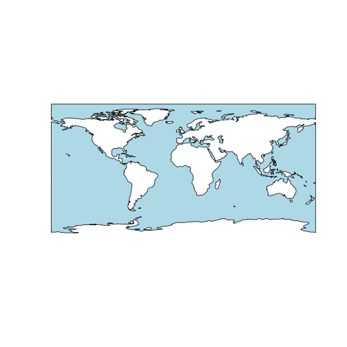
Cultural vector data
data(df_layers_cultural)

knitr::kable(
  df_layers_cultural,
  caption = "cultural vector data available via ne_download()"
)| layer | scale10 | scale50 | scale110 |
|---|---|---|---|
| admin_0_antarctic_claim_limit_lines | 1 | 0 | 0 |
| admin_0_antarctic_claims | 1 | 0 | 0 |
| admin_0_boundary_lines_disputed_areas | 1 | 1 | 0 |
| admin_0_boundary_lines_land | 1 | 1 | 1 |
| admin_0_boundary_lines_map_units | 1 | 0 | 0 |
| admin_0_boundary_lines_maritime_indicator | 1 | 1 | 0 |
| admin_0_boundary_map_units | 0 | 1 | 0 |
| admin_0_breakaway_disputed_areas | 0 | 1 | 0 |
| admin_0_countries | 1 | 1 | 1 |
| admin_0_countries_lakes | 1 | 1 | 1 |
| admin_0_disputed_areas | 1 | 0 | 0 |
| admin_0_disputed_areas_scale_rank_minor_islands | 1 | 0 | 0 |
| admin_0_label_points | 1 | 0 | 0 |
| admin_0_map_subunits | 1 | 1 | 0 |
| admin_0_map_units | 1 | 1 | 1 |
| admin_0_pacific_groupings | 1 | 1 | 1 |
| admin_0_scale_rank | 1 | 1 | 1 |
| admin_0_scale_rank_minor_islands | 1 | 0 | 0 |
| admin_0_seams | 1 | 0 | 0 |
| admin_0_sovereignty | 1 | 1 | 1 |
| admin_0_tiny_countries | 0 | 1 | 1 |
| admin_0_tiny_countries_scale_rank | 0 | 1 | 0 |
| admin_1_label_points | 1 | 0 | 0 |
| admin_1_seams | 1 | 0 | 0 |
| admin_1_states_provinces | 1 | 1 | 1 |
| admin_1_states_provinces_lakes | 1 | 1 | 1 |
| admin_1_states_provinces_lines | 1 | 1 | 1 |
| admin_1_states_provinces_scale_rank | 1 | 1 | 1 |
| airports | 1 | 1 | 0 |
| parks_and_protected_lands_area | 1 | 0 | 0 |
| parks_and_protected_lands_line | 1 | 0 | 0 |
| parks_and_protected_lands_point | 1 | 0 | 0 |
| parks_and_protected_lands_scale_rank | 1 | 0 | 0 |
| populated_places | 1 | 1 | 1 |
| populated_places_simple | 1 | 1 | 1 |
| ports | 1 | 1 | 0 |
| railroads | 1 | 0 | 0 |
| railroads_north_america | 1 | 0 | 0 |
| roads | 1 | 0 | 0 |
| roads_north_america | 1 | 0 | 0 |
| time_zones | 1 | 0 | 0 |
| urban_areas | 1 | 1 | 0 |
| urban_areas_landscan | 1 | 0 | 0 |
plot(
  ne_download(
    type = "airports",
    category = "cultural",
    scale = 10L
  )["geometry"],
  pch = 21L,
  bg = "grey"
)
#> Reading 'ne_10m_airports.zip' from naturalearth...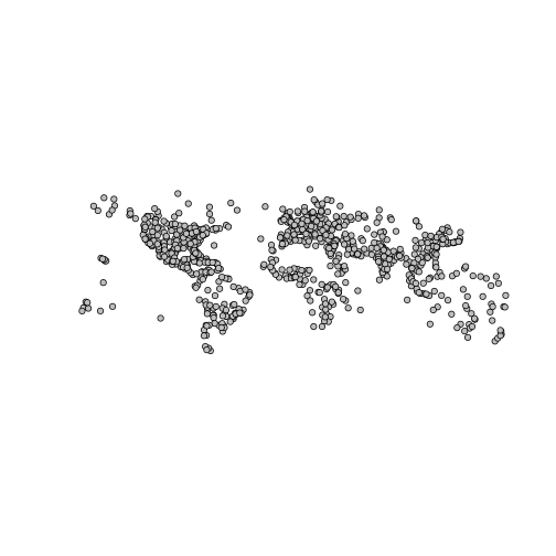
Searching for countries and continents
In this article, we explore how we can search for data available to
download within rnaturalearth. Let’s begin by loading
country data using the read_sf() function from the
sf package. In the following code snippet, we read the
Natural Earth dataset, which contains information about the sovereignty
of countries.
df <- read_sf(
"/vsizip/vsicurl/https://naciscdn.org/naturalearth/10m/cultural/ne_10m_admin_0_sovereignty.zip"
)
head(df)
#> Simple feature collection with 6 features and 168 fields
#> Geometry type: MULTIPOLYGON
#> Dimension: XY
#> Bounding box: xmin: -109.4537 ymin: -55.9185 xmax: 140.9776 ymax: 7.35578
#> Geodetic CRS: WGS 84
#> # A tibble: 6 × 169
#> featurecla scalerank LABELRANK SOVEREIGNT SOV_A3 ADM0_DIF LEVEL TYPE TLC ADMIN ADM0_A3
#> <chr> <int> <int> <chr> <chr> <int> <int> <chr> <chr> <chr> <chr>
#> 1 Admin-0 sover… 5 2 Indonesia IDN 0 2 Sove… 1 Indo… IDN
#> 2 Admin-0 sover… 5 3 Malaysia MYS 0 2 Sove… 1 Mala… MYS
#> 3 Admin-0 sover… 0 2 Chile CHL 0 2 Sove… 1 Chile CHL
#> 4 Admin-0 sover… 0 3 Bolivia BOL 0 2 Sove… 1 Boli… BOL
#> 5 Admin-0 sover… 0 2 Peru PER 0 2 Sove… 1 Peru PER
#> 6 Admin-0 sover… 0 2 Argentina ARG 0 2 Sove… 1 Arge… ARG
#> # ℹ 158 more variables: GEOU_DIF <int>, GEOUNIT <chr>, GU_A3 <chr>, SU_DIF <int>,
#> # SUBUNIT <chr>, SU_A3 <chr>, BRK_DIFF <int>, NAME <chr>, NAME_LONG <chr>, BRK_A3 <chr>,
#> # BRK_NAME <chr>, BRK_GROUP <chr>, ABBREV <chr>, POSTAL <chr>, FORMAL_EN <chr>,
#> # FORMAL_FR <chr>, NAME_CIAWF <chr>, NOTE_ADM0 <chr>, NOTE_BRK <chr>, NAME_SORT <chr>,
#> # NAME_ALT <chr>, MAPCOLOR7 <int>, MAPCOLOR8 <int>, MAPCOLOR9 <int>, MAPCOLOR13 <int>,
#> # POP_EST <dbl>, POP_RANK <int>, POP_YEAR <int>, GDP_MD <int>, GDP_YEAR <int>,
#> # ECONOMY <chr>, INCOME_GRP <chr>, FIPS_10 <chr>, ISO_A2 <chr>, ISO_A2_EH <chr>,
#> # ISO_A3 <chr>, ISO_A3_EH <chr>, ISO_N3 <chr>, ISO_N3_EH <chr>, UN_A3 <chr>, WB_A2 <chr>,
#> # WB_A3 <chr>, WOE_ID <int>, WOE_ID_EH <int>, WOE_NOTE <chr>, ADM0_ISO <chr>,
#> # ADM0_DIFF <chr>, ADM0_TLC <chr>, ADM0_A3_US <chr>, ADM0_A3_FR <chr>, ADM0_A3_RU <chr>,
#> # ADM0_A3_ES <chr>, ADM0_A3_CN <chr>, ADM0_A3_TW <chr>, ADM0_A3_IN <chr>, ADM0_A3_NP <chr>,
#> # ADM0_A3_PK <chr>, ADM0_A3_DE <chr>, ADM0_A3_GB <chr>, ADM0_A3_BR <chr>, ADM0_A3_IL <chr>,
#> # ADM0_A3_PS <chr>, ADM0_A3_SA <chr>, ADM0_A3_EG <chr>, ADM0_A3_MA <chr>, ADM0_A3_PT <chr>,
#> # ADM0_A3_AR <chr>, ADM0_A3_JP <chr>, ADM0_A3_KO <chr>, ADM0_A3_VN <chr>, ADM0_A3_TR <chr>,
#> # ADM0_A3_ID <chr>, ADM0_A3_PL <chr>, ADM0_A3_GR <chr>, ADM0_A3_IT <chr>, ADM0_A3_NL <chr>,
#> # ADM0_A3_SE <chr>, ADM0_A3_BD <chr>, ADM0_A3_UA <chr>, ADM0_A3_UN <int>, ADM0_A3_WB <int>,
#> # CONTINENT <chr>, REGION_UN <chr>, SUBREGION <chr>, REGION_WB <chr>, NAME_LEN <int>,
#> # LONG_LEN <int>, ABBREV_LEN <int>, TINY <int>, HOMEPART <int>, MIN_ZOOM <dbl>,
#> # MIN_LABEL <dbl>, MAX_LABEL <dbl>, LABEL_X <dbl>, LABEL_Y <dbl>, NE_ID <dbl>,
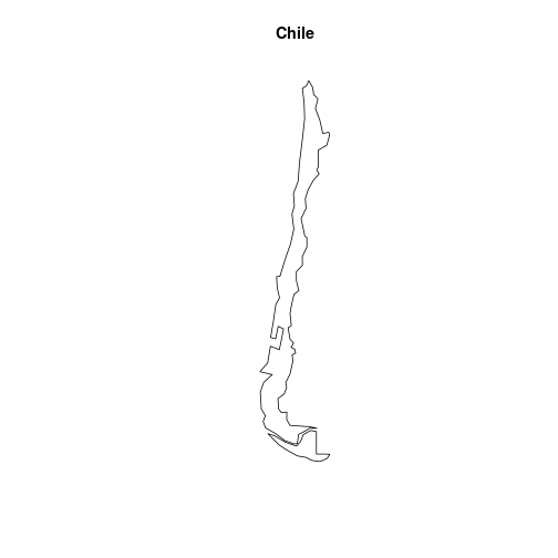
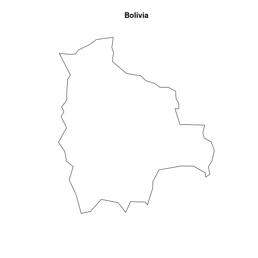
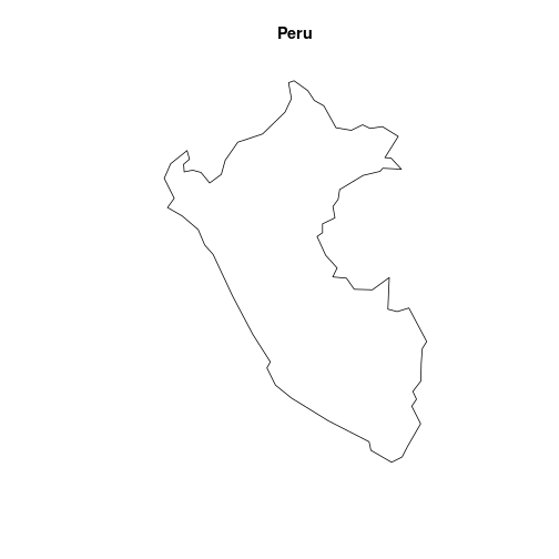
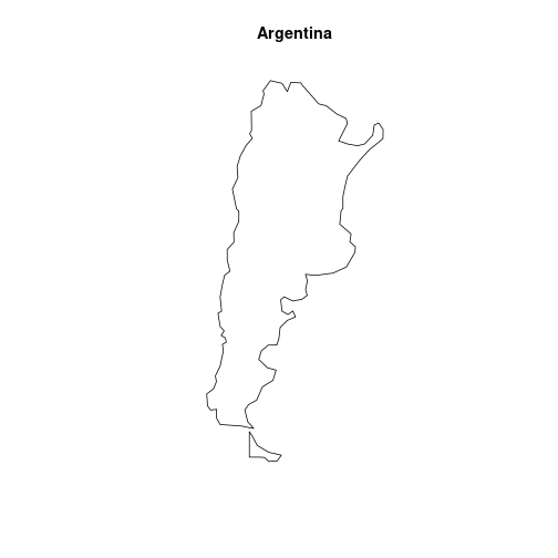
#> # WIKIDATAID <chr>, NAME_AR <chr>, NAME_BN <chr>, NAME_DE <chr>, …Finding countries
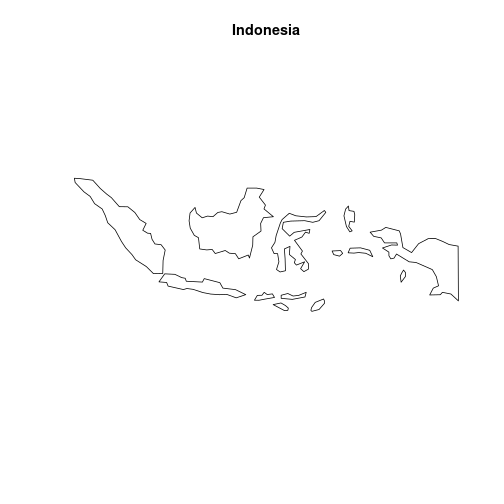
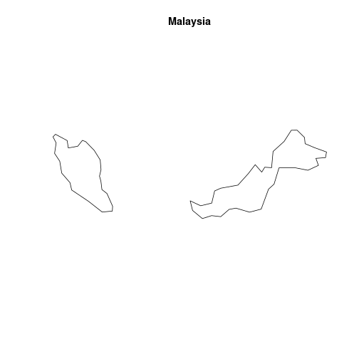
One way to search for countries is to search within the
ADMIN vector. Let’s start by plotting some of the first
countries.
lapply(
  df$ADMIN[1L:6L],
  \(x) plot(ne_countries(country = x)["geometry"], main = x)
)
Suppose that we want to search the polygons for the US, how should we spell it?
ne_countries(country = "USA")
ne_countries(country = "United States")
ne_countries(country = "United States Of America")
ne_countries(country = "United States of America")
One possibility consists to search within the ADMIN
vector using a regular expression to find all occurrences of the word
states.
grep("states", df$ADMIN, ignore.case = TRUE, value = TRUE)
#> [1] "United States of America"       "Federated States of Micronesia"
We can now get the data.
plot(ne_countries(country = "United States of America")["geometry"])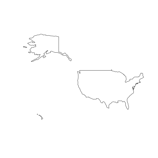
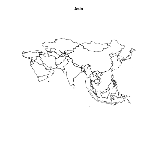
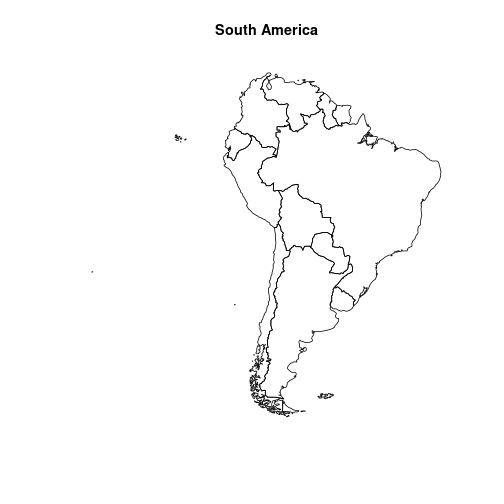
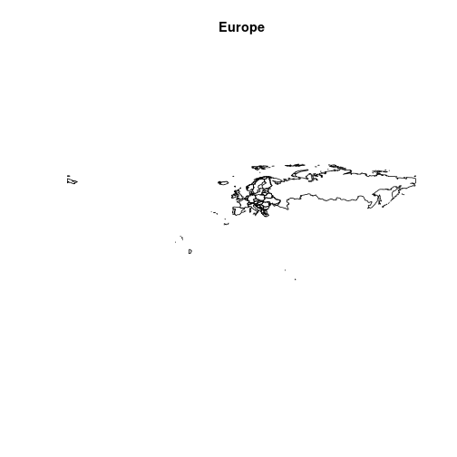
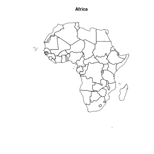
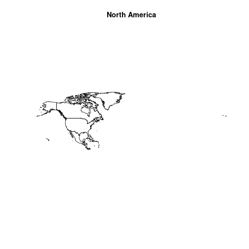
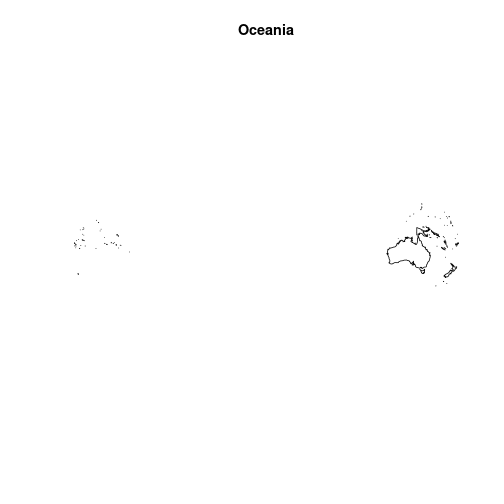
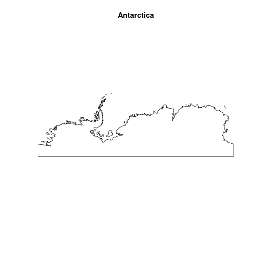
Continents
Finally, let’s create plots for each continent using the
ne_countries function with the continent parameter.
unique(df$CONTINENT)
#> [1] "Asia"                    "South America"           "Europe"
#> [4] "Africa"                  "North America"           "Oceania"
#> [7] "Antarctica"              "Seven seas (open ocean)"
lapply(
  unique(df$CONTINENT),
  \(x)
    plot(
      ne_countries(
        continent = x,
        scale = "medium"
      )["geometry"],
      main = x
    )
)