For forms with spatial types, such as geopoint, geotrace, or
geoshape, ruODK gives two options to access the captured
spatial data.
Firstly, to make spatial data as simple and accessible as possible,
ruODK extracts the lat/lon/alt/acc from geopoints, as well
as from the first coordinate of geotraces and geoshapes into separate
columns. This works for both GeoJSON and WKT. The extracted columns are
named as the original geofield appended with _latitude,
_longitude, _altitude, and
_accuracy, respectively.
Secondly, this vignette demonstrates how to turn the spatial data types returned from ODK Central into spatially enabled objects. To do so, we have to address two challenges.
The first challenge is to select which of the potentially many
spatial fields which an ODK form can capture shall be used as the
primary geometry of a native spatial object, such as an sf
SimpleFeature class. If several spatial fields are captured, it is up to
the user to choose which field to use as primary geometry.
The second challenge is that the parsed data from ODK Central is a
plain table (tbl_df) in which some columns contain spatial
data. Well Know Text (WKT) is parsed as text columns, whereas GeoJSON
(nested JSON) is parsed as list columns.
Most spatial packages require either atomic coordinates in separate
columns, which works well for points (latitude, longitude, altitude), or
the data to be spatially enabled. This vignette shows how to transform a
tbl_df with a column containing (point, line, or polygon)
WKT into a spatially enabled sf object.
library(ruODK)

# Visualisation
library(leaflet)
library(ggplot2)
library(lattice)
# library(tmap) # Suggested but not included here yet

# Spatial
can_run <- require(sf) && require(leafem) && require(mapview) && require(terra)
# Fix https://github.com/r-spatial/mapview/issues/313
# See also https://github.com/r-spatial/mapview/issues/312
# option 'fgb' requires GDAL >= 3.1.0
if (require(mapview)) {
  mapview::mapviewOptions(
    fgb = FALSE,
    basemaps = c(
      "Esri.WorldImagery",
      "Esri.WorldShadedRelief",
      "OpenTopoMap",
      "OpenStreetMap"
    ),
    layers.control.pos = "topright"
  )
}
Data
The original data shown in this vignette are hosted on a ODK Central
server which is used for the ruODK package tests. The form
we show here contains every spatial widget supported by ODK Build for
every supported spatial field type.
With working credentials to the ODK Central test server we could download the data directly.
# Set ruODK defaults to an ODK Central form, choose tz and verbosity
ruODK::ru_setup(
  url = get_test_url(),
  pid = get_test_pid(),
  fid = get_test_fid_wkt(),
  un = get_test_un(),
  pw = get_test_pw(),
  odkc_version = "2023.5.1",
  tz = "Australia/Perth",
  verbose = TRUE
)
data_wkt <- ruODK::odata_submission_get(wkt = TRUE)
data_gj <- ruODK::odata_submission_get(wkt = FALSE)
To allow users to build this vignette without credentials to the ODK
Central test server, ruODK provides above form data also as
package data.
Map geopoints
We can turn data with a text column containing WKT into an
sf (SimpleFeatures) object.
In addition, we can leave the tbl_df as non-spatial
object, and instead use the separately extracted latitude, longitude,
altitude, and accuracy individually e.g. to plot a Leaflet map.
geo_sf_point <- geo_wkt %>% sf::st_as_sf(wkt = "point_location_point_gps")
# ODK Collect captures WGS84 (EPSG:4326)
sf::st_crs(geo_sf_point) <- 4326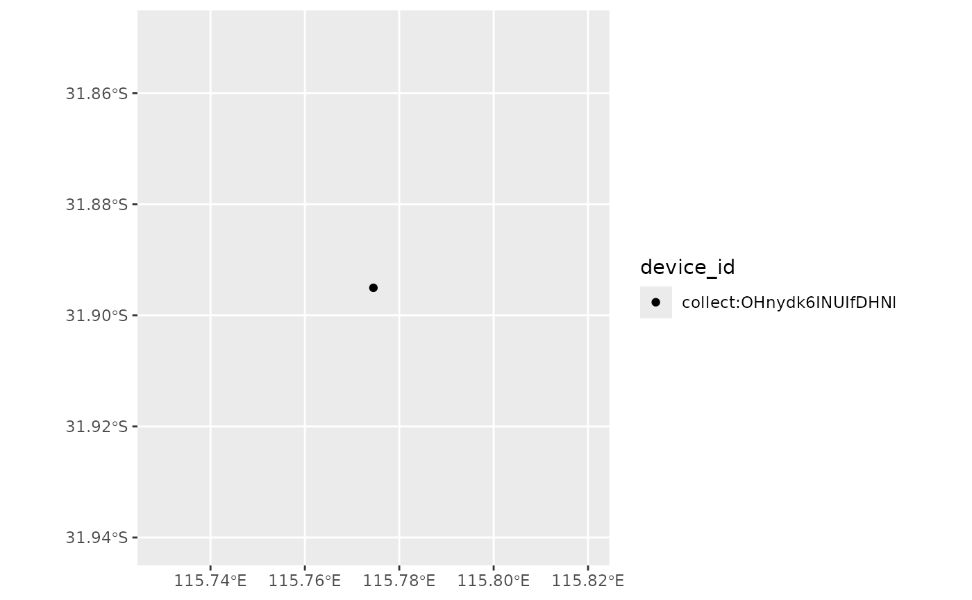
Leaflet using sf
leaflet::leaflet(data = geo_sf_point) %>%
  leaflet::addTiles() %>%
  leaflet::addMarkers(label = ~device_id, popup = ~device_id)
Leaflet using extracted coordinate components in tbl_df
leaflet::leaflet(data = geo_wkt) %>%
  leaflet::addTiles() %>%
  leaflet::addMarkers(
    lng = ~point_location_point_gps_longitude,
    lat = ~point_location_point_gps_latitude,
    label = ~device_id,
    popup = ~device_id
  )
Map geotraces (lines)
We use sf::st_as_sf on a text column containing a WKT
geotrace.
geo_sf_line <- geo_wkt %>% sf::st_as_sf(wkt = "path_location_path_gps")
# ODK Collect captures WGS84 (EPSG:4326)
sf::st_crs(geo_sf_line) <- 4326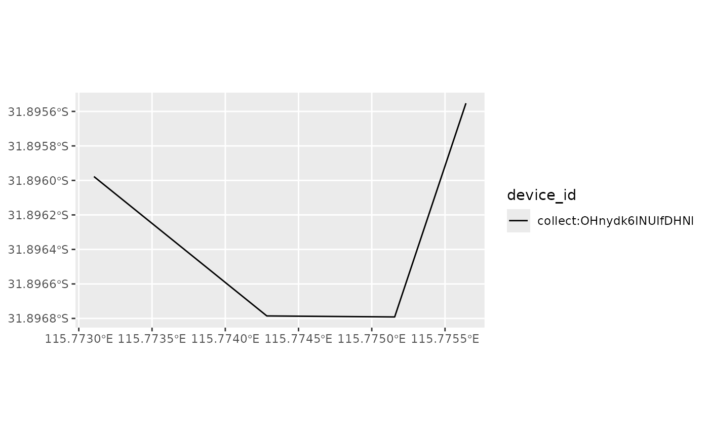
Leaflet using sf and extracted coordinates
You can show either first extracted coordinate components from plain
tbl_df or show the full polygons using
leafem. See the mapview article on extra
functionality.
leaflet::leaflet(data = geo_wkt) %>%
  leaflet::addTiles() %>%
  leaflet::addMarkers(
    lng = ~path_location_path_gps_longitude,
    lat = ~path_location_path_gps_latitude,
    label = ~device_id,
    popup = ~device_id
  ) %>%
  leafem::addFeatures(geo_sf_line, label = ~device_id, popup = ~device_id)
Map geoshapes (polygons)
Again, we’ll use sf::st_as_sf but select a WKT geoshape
column.
geo_sf_poly <- geo_wkt %>% sf::st_as_sf(wkt = "shape_location_shape_gps")
# ODK Collect captures WGS84 (EPSG:4326)
sf::st_crs(geo_sf_poly) <- 4326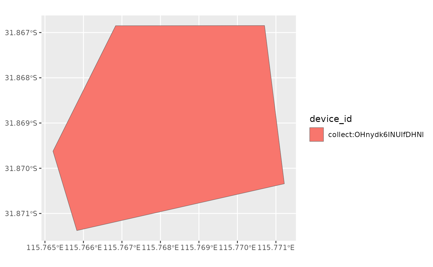
Leaflet using sf and extracted coordinates
You can show either first extracted coordinate components from plain
tbl_df or show the full polygons using
leafem. See the mapview article on extra
functionality.
leaflet::leaflet(data = geo_wkt) %>%
  leaflet::addTiles() %>%
  leaflet::addMarkers(
    lng = ~shape_location_shape_gps_longitude,
    lat = ~shape_location_shape_gps_latitude,
    label = ~device_id,
    popup = ~device_id
  ) %>%
  leafem::addFeatures(geo_sf_poly, label = ~device_id, popup = ~device_id)
Outlook
The above examples show how to turn spatial data into an
sf object, and give very rudimentary visualisation examples
to bridge the gap between spatial data coming from ODK and creating maps
and further spatial analyses in R.
See the sf homepage for more context and examples. The sf cheatsheet deserves a spatial mention.
Review the options for mapview popups and the whole mapview homepage for a comprehensive overview of mapview.
The powerful visualisation package tmap
supports sf objects and produces both printable and static
maps as well as interactive leaflet maps. See the vignette
“Get started”.
There are several other good entry points for all things R and spatial, including but not limited to:
- The R Spatial CRAN Task View
- The RSpatial website
- Geospatial data in R and beyond by Barry Rowlingson
- GIS with R by Jesse Sadler
- GIS and mapping by Olivier Gimenez: Slides and code
The above list of examples and resources is far from comprehensive.
Feel free to contribute or
suggest other working examples for turning data from
ruODK into spatial formats.