Introduction
This article aims to provide external verification of the results provided by the package. So far only one verification dataset has been used, but we hope to find others. If you know of verification datasets, please let us know — initially we planned to use a dataset from a paper on river slopes (Cohen et al. 2018), but we could find no way of extracting the underlying data to do the calculation.
For this article we primarily used the following packages, although others are loaded in subsequent code chunks.
The results are reproducible (requires downloading input data manually and installing additional packages). To keep package build times low, only the results are presented below.
Case studies
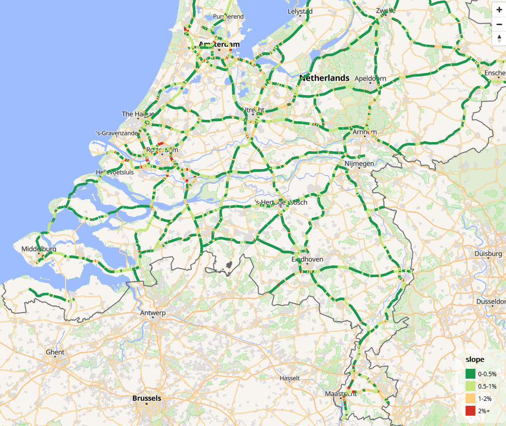
Roads in the Netherlands
u = "https://downloads.rijkswaterstaatdata.nl/nwb-wegen/geogegevens/shapefile/NWB_hoogtebestand/01-10-2024%20Hoogtes_Rijkswegen.zip"
f_zip = "NWB_hoogtebestand.zip"
if (!file.exists(f_zip)) {
  download.file(u, f_zip)
  unzip(f_zip)
  # Datasets in
  list.files("NWB3D_resultaten_oktober_2024.gdb")
  roads_nl_layers = sf::st_layers("NWB3D_resultaten_oktober_2024.gdb")
#   Driver: OpenFileGDB
# Available layers:
#                                   layer_name        geometry_type features
# 1    NWB3D_resultaten_oktober_2024_wegvakken 3D Multi Line String    16456
# 2 NWB3D_resultaten_oktober_2024_vertexpunten             3D Point  1095615
#   fields            crs_name
# 1     59 Amersfoort / RD New
# 2     59 Amersfoort / RD New
  roads_nl = sf::st_read("NWB3D_resultaten_oktober_2024.gdb", layer = "NWB3D_resultaten_oktober_2024_wegvakken")
  names(roads_nl)
#    [1] "WVK_ID"        "BST_CODE"      "WVK_BEGDAT"    "JTE_ID_BEG"
#  [5] "JTE_ID_END"    "WEGBEHSRT"     "WEGNUMMER"     "WEGDEELLTR"
#  [9] "HECTO_LTTR"    "RPE_CODE"      "ADMRICHTNG"    "RIJRICHTNG"
# [13] "STT_NAAM"      "STT_BRON"      "WPSNAAM"       "GME_ID"
# [17] "GME_NAAM"      "HNRSTRLNKS"    "HNRSTRRHTS"    "E_HNR_LNKS"
# [21] "E_HNR_RHTS"    "L_HNR_LNKS"    "L_HNR_RHTS"    "BEGAFSTAND"
# [25] "ENDAFSTAND"    "BEGINKM"       "EINDKM"        "POS_TV_WOL"
# [29] "WEGBEHCODE"    "WEGBEHNAAM"    "DISTRCODE"     "DISTRNAAM"
# [33] "DIENSTCODE"    "DIENSTNAAM"    "WEGTYPE"       "WGTYPE_OMS"
# [37] "ROUTELTR"      "ROUTENR"       "ROUTELTR2"     "ROUTENR2"
# [41] "ROUTELTR3"     "ROUTENR3"      "ROUTELTR4"     "ROUTENR4"
# [45] "WEGNR_AW"      "WEGNR_HMP"     "GEOBRON_ID"    "GEOBRON_NM"
# [49] "BRONJAAR"      "OPENLR"        "BAG_ORL"       "FRC"
# [53] "FOW"           "ALT_NAAM"      "ALT_NR"        "REL_HOOGTE"
# [57] "Hoogte_bron"   "Kwaliteitlaag" "SHAPE_Length"  "SHAPE"
# Plot the slopes (variable called REL_HOOGTE):
  summary(roads_nl$REL_HOOGTE)
  # xyz
  roads_nl_xyz = sf::st_coordinates(roads_nl)
  head(roads_nl_xyz)
  hist(roads_nl_xyz[, "Z"], breaks = 50, main = "Histogram of elevation values (m)", xlab = "Elevation (m)")
  plot(roads_nl["REL_HOOGTE"])
  summary(sf::st_geometry_type(roads_nl))
  roads_nl$slope = roads_nl |>
    sf::st_cast("LINESTRING") |>
    slopes::slope_xyz() * 100

  summary(roads_nl$slope)
  library(tmap)
  library(tmap.mapgl)
  m = tm_shape(roads_nl) +
    tm_lines(
      col = "slope",
      col.scale = tm_scale_intervals(
        breaks = c(-1, 0.5, 1, 2, 20),
        labels = c("0-0.5%", "0.5-1%", "1-2%", "2%+"),
        values = cols4all::c4a("-brewer.rd_yl_gn")
      ),
      lwd = 5
  )
  tmap_mode("maplibre")
  m
}
Comparison of DEM-derived and survey-grade Z values
The NL NWB Hoogtebestand contains 3D linestring geometries with Z
coordinates derived from high-resolution Dutch elevation models
(AHN4/AHN5, with sub-10 cm vertical accuracy). These provide a ground
truth against which the slopes package’s DEM-derived
elevation estimates can be compared, as proposed in issue #71.
The following code demonstrates the comparison, using a sample of 30
road segments from South Limburg (the hilliest region of the
Netherlands, with elevations ranging from 32 m to 181 m above NAP) and
an independent DEM sourced from AWS Open Data terrain tiles via the
elevatr package (zoom level 10, approximately 120 m
resolution).
# Load the NL data (see code above) and focus on South Limburg
roads_wgs84 = sf::st_transform(roads_nl, 4326)
coords_centroid = sf::st_coordinates(sf::st_centroid(st_geometry(roads_wgs84)))
in_limburg = coords_centroid[, "Y"] > 50.75 &
             coords_centroid[, "Y"] < 51.0 &
             coords_centroid[, "X"] > 5.6 &
             coords_centroid[, "X"] < 6.1
roads_limburg = roads_nl[in_limburg, ]

# Pick 30 segments with most Z variation
get_z_range = function(geom) {
  c = sf::st_coordinates(geom)
  if (nrow(c) < 2) return(0)
  diff(range(c[, "Z"]))
}
z_ranges = sapply(sf::st_geometry(roads_limburg), get_z_range)
top_idx = order(z_ranges, decreasing = TRUE)[1:30]
roads_sample = roads_limburg[top_idx, ]

# Download DEM via elevatr (AWS Open Data, no API key required)
library(elevatr)
roads_sample_wgs84 = sf::st_transform(roads_sample, 4326)
bb = sf::st_bbox(roads_sample_wgs84)
# Buffer the bbox by ~1 km to ensure all vertices are covered
bb_mat = matrix(c(
  bb["xmin"] - 0.01, bb["ymin"] - 0.01,
  bb["xmax"] + 0.01, bb["ymin"] - 0.01,
  bb["xmax"] + 0.01, bb["ymax"] + 0.01,
  bb["xmin"] - 0.01, bb["ymax"] + 0.01,
  bb["xmin"] - 0.01, bb["ymin"] - 0.01
), ncol = 2, byrow = TRUE)
bb_sf = sf::st_sf(geometry = sf::st_sfc(sf::st_polygon(list(bb_mat)), crs = 4326))
dem_elevatr = get_elev_raster(bb_sf, z = 10, clip = "bbox")
# Project DEM to match the NL data CRS (EPSG:28992)
dem_28992 = terra::project(terra::rast(dem_elevatr), "EPSG:28992", method = "bilinear")

# Prepare roads: cast to LINESTRING and record actual Z values
roads_ls = sf::st_cast(roads_sample, "LINESTRING")
coords_before = sf::st_coordinates(roads_ls)
actual_z = coords_before[, "Z"]

# Add elevation from the DEM using the slopes package
roads_with_z = slopes::elevation_add(roads_ls, dem = dem_28992)
coords_after = sf::st_coordinates(roads_with_z)
est_z = coords_after[, "Z"]

# Compare Z values
z_diff = est_z - actual_z
cat("Z RMSE:", round(sqrt(mean(z_diff^2)), 2), "m\n")
cat("Z MAE:", round(mean(abs(z_diff)), 2), "m\n")
cat("Z correlation (r):", round(cor(est_z, actual_z), 3), "\n")
cat("Z mean bias:", round(mean(z_diff), 2), "m\n")

# Compare slopes (both in EPSG:28992, so lonlat = FALSE)
slopes_actual = slopes::slope_xyz(roads_ls, lonlat = FALSE) * 100
slopes_est = slopes::slope_xyz(roads_with_z, lonlat = FALSE) * 100
cat("Slope correlation (r):",
    round(cor(slopes_actual, slopes_est, use = "complete.obs"), 3), "\n")
cat("Slope RMSE:",
    round(sqrt(mean((slopes_est - slopes_actual)^2, na.rm = TRUE)), 3), "%\n")
The results of this comparison, based on 7458 vertices across 30 road segments in South Limburg, are summarised below.
| Metric | Elevation (Z) | Slope (%) |
|---|---|---|
| RMSE | 4.78 m | 0.805 |
| MAE | 3.59 m | 0.586 |
| Correlation (r) | 0.989 | 0.802 |
| Mean bias | -0.67 m | +0.14 |
The elevation estimates from the DEM are very strongly correlated
with the survey-grade NL road heights (r = 0.989, RMSE = 4.78 m),
demonstrating that the slopes package’s
elevation_add() function accurately captures the general
terrain. The slight negative bias (-0.67 m) and the RMSE of under 5 m
are consistent with the expected vertical accuracy of the AWS terrain
tiles at this zoom level.
The slope estimates are also well correlated (r = 0.802), with a modest RMSE of 0.81%. The DEM-derived slopes have a lower maximum (5.5% vs 7.3%) and lower standard deviation (1.16% vs 1.34%) than the NL data, reflecting the smoothing effect of the coarser DEM resolution. This is consistent with the findings from the GNSS trace comparison above: the package provides less noisy slope estimates than raw GPS data, but may underestimate steeper gradients due to DEM resolution limitations.
DEM for eu:
install.packages(“CopernicusDEM”) system(“msiexec.exe /i https://awscli.amazonaws.com/AWSCLIV2.msi”) # Test it’s
installed: system(“aws –version”) # Find location of aws cli from
powershell (equivalent of which aws on Linux): #
Get-Command aws | Select-Object -ExpandProperty Source # C:Files.exe
current_path = Sys.getenv(“PATH”)
aws_path = “C:\Program Files\Amazon\AWSCLIV2” new_path = paste(aws_path, current_path, sep = “;”) Sys.setenv(PATH = new_path) # Now aws should work system(“aws –version”) # Download DEM for Brussels 6 km from center zones = zonebuilder::zb_zone(“Brussels”, n_circles = 3) region = sf::st_union(zones$geometry) |> sf::st_make_valid() sf::sf_use_s2(TRUE) # disable s2 for this operation region_plus_100m = sf::st_buffer(region, dist = 100) mapview::mapview(region) + mapview::mapview(region_plus_100m) sf::sf_use_s2(FALSE) # disable s2 for this operation dir_save_tifs = "dems-brussels" dem = CopernicusDEM::aoi_geom_save_tif_matches( sf_or_file = region_plus_100m, dir_save_tifs = dir_save_tifs, resolution = 30, crs_value = 4326, threads = parallel::detectCores(), verbose = TRUE ) dems = list.files(dir_save_tifs, full.names = TRUE) dem_terra = terra::rast(dems) names(dem_terra) dem_cropped = terra::crop(dem_terra, region_plus_100m) mapview::mapview(dem_cropped) travel_network = osmactive::get_travel_network( region, boundary = region, boundary_type = "clipsrc" ) plot(travel_network$geometry) travel_network = travel_network |> sf::st_filter(region, .predicate = sf::st_within)
cycle_net = osmactive::get_cycling_network(travel_network) drive_net = osmactive::get_driving_network(travel_network) cycle_net = osmactive::distance_to_road(cycle_net, drive_net) cycle_net = osmactive::classify_cycle_infrastructure(cycle_net, include_mixed_traffic = TRUE) names(cycle_net) mapview::mapview(cycle_net, zcol = “cycle_segregation”) nrow(cycle_net) # Calculate slopes with the slopes package: # Add elevation to cycle network segments
sf::st_crs(dem_cropped) == sf::st_crs(cycle_net) # check the extents of both: mapview::mapview(dem_cropped) + mapview::mapview(cycle_net)
cycle_net_clean = sf::st_cast(cycle_net, “LINESTRING”) cycle_net_xyz = elevation_add(cycle_net_clean, dem = dem_cropped) summary(sf::st_geometry_type(cycle_net_xyz))
Calculate slopes for each segment
cycle_net_xyz$slope = slope_xyz(cycle_net_xyz, lonlat = TRUE, fun = slope_matrix_weighted) # cycle_net_xyz$slope = slope_xyz(cycle_net_xyz, lonlat = TRUE, fun = slope_matrix_mean) summary(cycle_net_xyz$slope) # Convert to percentage: cycle_net_xyz = cycle_net_xyz |> # Convert to factor with greater than 5 being "5+" dplyr::mutate( slope_percent = dplyr::case_when( slope < 0.02 ~ as.character("0-2"), slope < 0.05 ~ as.character("2-5"), slope < 0.08 ~ as.character("5-8"), TRUE ~ "8+" ) ) table(cycle_net_xyz$slope_percent)
Drop z dimension
cycle_net_slopes = sf::st_zm(cycle_net_xyz) |> dplyr::transmute(osm_id, highway, cycle_segregation, slope = round(slope, 3), slope_percent) summary(duplicated(cycle_net_slopes$geometry)) mapview::mapview(cycle_net_slopes, zcol = “slope_percent”, legend = TRUE) sf::write_sf(cycle_net_slopes, “cycle_net_slopes_brussels.gpkg”, delete_dsn = TRUE) system(“gh release upload v1.0.1 cycle_net_slopes_brussels.gpkg –clobber”) cycle_net_slopes = sf::read_sf(“cycle_net_slopes_brussels.gpkg”)
install cran version
remotes::install_dev(“tmap”) # Save with tmap library(tmap) v = cols4all::c4a(“brewer.rd_yl_gn”, n = 4) |> rev() m = tm_shape(cycle_net_slopes) + tm_lines( col = “slope_percent”, col.scale = tm_scale(values = v), lwd = 2, popup.vars = FALSE ) m tmap_save(m, “cycle_net_slopes_brussels.html”) browseURL(“cycle_net_slopes_brussels.html”) system(“gh release upload v1.0.1 cycle_net_slopes_brussels.html –clobber”) # url of the file: u_release = “https://github.com/ropensci/slopes/releases/download/v1.0.1/cycle_net_slopes_brussels.html” download.file(u_release, “cycle_net_slopes_brussels.html”)
# Comparison with results from ArcMap 3D Analyst
# Three-dimensional traces of roads dataset
<!-- todo: make the segments -->
An input dataset, comprising a 3D linestring recorded using a dual frequency GNSS receiver (a [Leica 1200](https://gef.nerc.ac.uk/equipment/gnss/)) with a vertical accuracy of 20 mm
<!-- 138 GPS 3D traces of a hilly road from a peer reviewed journal article -->
[@ariza-lopez_dataset_2019] was downloaded from the
<!-- [figshare website as a .zip file](https://ndownloader.figshare.com/files/14331197) - raw data -->
[figshare website as a .zip file](https://ndownloader.figshare.com/files/14331185)
and unzipped and inflated in the working directory as follows (not evaluated to reduce package build times):
``` r
download.file("https://ndownloader.figshare.com/files/14331185", "3DGRT_AXIS_EPSG25830_v2.zip")
unzip("3DGRT_AXIS_EPSG25830_v2.zip")
trace = sf::read_sf("3DGRT_AXIS_EPSG25830_v2.shp")
plot(trace)
nrow(trace)
#> 11304
summary(trace$X3DGRT_h)
#> Min. 1st Qu. Median Mean 3rd Qu. Max.
#> 642.9 690.3 751.4 759.9 834.3 884.9 To verify our estimates of hilliness, we generated slope estimates for each segment and compared them with Table 7 in Ariza-López et al. (2019). The absolute gradient measure published in that paper were:
res_gps = c(0.00, 4.58, 1136.36, 6.97)
res_final = c(0.00, 4.96, 40.70, 3.41)
res = data.frame(cbind(
  c("GPS", "Dual frequency GNSS receiver"),
  rbind(res_gps, res_final)
))
names(res) = c("Source", "min", " mean", " max", " stdev")
knitr::kable(res, row.names = FALSE)| Source | min | mean | max | stdev |
|---|---|---|---|---|
| GPS | 0 | 4.58 | 1136.36 | 6.97 |
| Dual frequency GNSS receiver | 0 | 4.96 | 40.7 | 3.41 |
# mapview::mapview(trace) # check extent: it's above 6km in height
# remotes::install_github("hypertidy/ceramic")
loc = colMeans(sf::st_coordinates(sf::st_transform(trace, 4326)))
e = ceramic::cc_elevation(loc = loc[1:2], buffer = 3000)
trace_projected = sf::st_transform(trace, 3857)
plot(e)
plot(trace_projected$geometry, add = TRUE)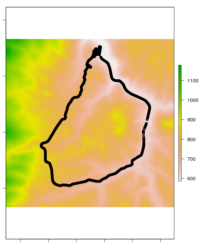
The slopes were estimated as follows:
# source: https://www.robinlovelace.net/presentations/munster.html#31
points2line_trajectory = function(p) {
  c = st_coordinates(p)
  i = seq(nrow(p) - 2)
  l = purrr::map(i, ~ sf::st_linestring(c[.x:(.x + 1), ]))
  lfc = sf::st_sfc(l)
  a = seq(length(lfc)) + 1 # sequence to subset
  p_data = cbind(sf::st_set_geometry(p[a, ], NULL))
  sf::st_sf(p_data, geometry = lfc)
}
r = points2line_trajectory(trace_projected)
# summary(st_length(r)) # mean distance is 1m! Doesn't make sense, need to create segments
s = slope_raster(r, e = e)
slope_summary = data.frame(min = min(s), mean = mean(s), max = max(s), stdev = sd(s))
slope_summary = slope_summary * 100
knitr::kable(slope_summary, digits = 1)| min | mean | max | stdev |
|---|---|---|---|
| 0 | 6.2 | 48.2 | 5.6 |
Combined with the previous table from Ariza-López et al. (2019), these results can be compared with those obtained from mainstream GPS, and an accurate GNSS receiver:
| Source | min | mean | max | stdev |
|---|---|---|---|---|
| GPS | 0 | 4.58 | 1136.36 | 6.97 |
| Dual frequency GNSS receiver | 0 | 4.96 | 40.7 | 3.41 |
| Slopes R package | 0 | 6.2 | 48.2 | 5.6 |
It is notable that the package substantially overestimates the gradient, perhaps due to the low resolution of the underlying elevation raster. However, the slopes package seems to provide less noisy slope estimates than the GPS approach, with lower maximum values and low standard deviation.