Analyzing work loop experiments in workloopR
Vikram B. Baliga
2026-07-01
Source:vignettes/Analyzing-workloops.Rmd
Analyzing-workloops.RmdThe function analyze_workloop() in
workloopR allows users to evaluate the mechanical work and
power output of a muscle they have investigated through work loop
experiments.
To demonstrate analyze_workloop(), we will first load
workloopR and use example data provided with the package.
We’ll also load a couple packages within the tidyverse to
help with data wrangling and plotting.
Visualize
We’ll now import the workloop.ddf file included with
workloopR. Because this experiment involved using a gear
ratio of 2, we’ll use fix_GR() to also implement this
correction.
Ultimately, an object of classes workloop,
muscle_stim, and data.frame is produced.
muscle_stim objects are used throughout
workloopR to help with data formatting and error checking
across functions. Additionally setting the class to
workloop allows our functions to understand that the data
have properties that other experiment types (twitch, tetanus) do
not.
## The file workloop.ddf is included and therefore can be accessed via
## system.file("subdirectory","file_name","package") . We'll then use
## read_ddf() to import it, creating an object of class "muscle_stim".
## fix_GR() multiplies Force by 2 and divides Position by 2
workloop_dat <-
  system.file(
    "extdata",
    "workloop.ddf",
    package = 'workloopR') %>%
  read_ddf(phase_from_peak = TRUE) %>%
  fix_GR(GR = 2)

summary(workloop_dat)
#> # Workloop Data: 3 channels recorded over 0.3244s
#>
#> File ID: workloop.ddf
#> Mod Time (mtime): 2026-07-01 08:15:20
#> Sample Frequency: 10000Hz
#>
#> data.frame Columns:
#>   Position (mm)
#>   Force (mN)
#>   Stim (TTL)
#>
#> Stimulus Offset: 0.012s
#> Stimulus Frequency: 300Hz
#> Stimulus Width: 0.2ms
#> Stimulus Pulses: 4
#> Gear Ratio: 2
#>
#> Cycle Frequency: 28Hz
#> Total Cycles (L0-to-L0): 6
#> Amplitude: 1.575mm
Running summary() on a `muscle_stim shows a handy
summary of file properties, data, and experimental parameters.
Let’s plot Time against Force, Position, and Stimulus (Stim) to visualize the time course of the work loop experiment.
To get them all plotted in the same figure, we’ll transform the data as they are being plotted. Please note that this is for aesthetic purposes only - the underlying data will not be changed after the plotting is complete.
scale_position_to_force <- 3000

workloop_dat %>%
  # Set the x axis for the whole plot
  ggplot(aes(x = Time)) +
  # Add a line for force
  geom_line(aes(y = Force, color = "Force"),
            lwd = 1) +
  # Add a line for Position, scaled to approximately the same range as Force
  geom_line(aes(y = Position * scale_position_to_force, color = "Position")) +
  # For stim, we only want to plot where stimulation happens, so we filter the data
  geom_point(aes(y = 0, color = "Stim"), size = 1,
             data = filter(workloop_dat, Stim == 1)) +
  # Next we add the second y-axis with the corrected units
  scale_y_continuous(sec.axis = sec_axis(~ . / scale_position_to_force, name = "Position (mm)")) +
  # Finally set colours, labels, and themes
  scale_color_manual(values = c("#FC4E2A", "#4292C6", "#373737")) +
  labs(y = "Force (mN)", x = "Time (secs)", color = "Parameter:") +
  ggtitle("Time course of \n work loop experiment") +
  theme_bw() +
  theme(legend.position = "bottom", legend.direction = "horizontal")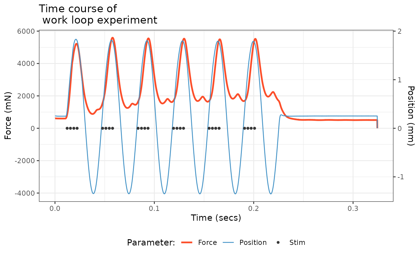
There’s a lot to digest here. The blue trace shows the change in length of the muscle via cyclical, sinusoidal changes to Position. The dark gray Stim dots show stimulation on a off vs. on basis. Stimulus onset is close to when the muscle is at L0 and the stimulator zapped the muscle four times in pulses of 0.2 ms width at 300 Hz. The resulting force development is shown in red. These cycles of length change and stimulation occurred a total of 6 times (measuring L0-to-L0).
Select cycles
We are now ready to run the select_cycles() function.
This function subsets the data and labels each cycle in prep for our
analyze_workloop() function.
In many cases, researchers are interested in using the final 3 cycles
for analyses. Accordingly, we’ll set the keep_cycles
parameter to 4:6.
One thing to pay heed to is the cycle definition, encoded as
cycle_def within the arguments of
select_cycles(). There are three options for how cycles can
be defined and are named based on the starting (and ending) points of
the cycle. We’ll use the L0-to-L0 option, which is encoded as
lo.
The function internally performs butterworth filtering of the
Position data via signal::butter(). This is because
Position data are often noisy, which makes assessing true peak values
difficult. The default values of bworth_order = 2 and
bworth_freq = 0.05 work well in most cases, but we
recommend you please plot your data and assess this yourself.
We will keep things straightforward for now so that we can proceed to
the analytical stage. Please see the final section of this vignette for
more details on using select_cycles().
## Select cycles
workloop_selected <-
  workloop_dat %>%
  select_cycles(cycle_def="lo", keep_cycles = 4:6)

summary(workloop_selected)
#> # Workloop Data: 4 channels recorded over 0.1086s
#>
#> File ID: workloop.ddf
#> Mod Time (mtime): 2026-07-01 08:15:20
#> Sample Frequency: 10000Hz
#>
#> data.frame Columns:
#>   Position (mm)
#>   Force (mN)
#>   Stim (TTL)
#>   Cycle (letters)
#>
#> Stimulus Offset: 0.012s
#> Stimulus Frequency: 300Hz
#> Stimulus Width: 0.2ms
#> Stimulus Pulses: 4
#> Gear Ratio: 2
#>
#> Cycle Frequency: 28Hz
#> Total Cycles (L0-to-L0): 6
#> Cycles Retained: 3
#> Amplitude: 1.575mm

attr(workloop_selected, "retained_cycles")
#> [1] 4 5 6
The summary() function now reflects that 3 cycles of the
original 6 have been retained, and getting the
"retained_cycles" attribute shows that these cycles are 4,
5, and 6 from the original data.
To avoid confusion in numbering schemes between the original data and
the new object, once select_cycles() has been used we label
cycles by letter. So, cycle 4 is now “a”, 5 is “b” and 6 is “c”.
Plot the work loop cycles
workloop_selected %>%
  ggplot(aes(x = Position, y = Force)) +
  geom_point(size=0.3) +
  labs(y = "Force (mN)", x = "Position (mm)") +
  ggtitle("Work loop") +
  theme_bw()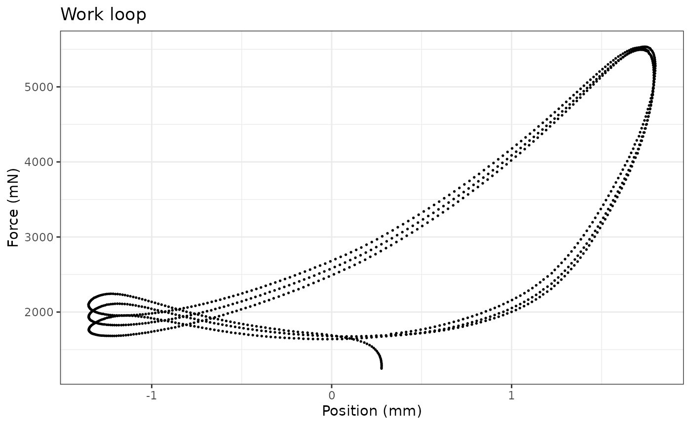
Basics of analyze_workloop()
Now we’re ready to use analyze_workloop().
Again, running select_cycles() beforehand was necessary,
so we will switch to using workloop_selected as our data
object.
Within analyze_workloop(), the GR = option
allows for the gear ratio to be corrected if it hasn’t been already. But
because we already ran fix_GR() to correct the gear ratio
to 2, we will not need to use it here again. So, this for this argument,
we will use GR = 1, which keeps the data as they are.
Please take care to ensure that you do not overcorrect for gear ratio by
setting it multiple times. Doing so induces multiplicative changes. E.g.
setting GR = 3 on an object and then setting
GR = 3 again produces a gear ratio correction of 9.
Using the default simplify = FALSE version
The argument simplify = affects the output of the
analyze_workloop() function. We’ll first take a look at the
organization of the “full” version, i.e. keeping the default
simplify = FALSE.
## Run the analyze_workloop() function
workloop_analyzed <-
  workloop_selected %>%
  analyze_workloop(GR = 1)

## Produces a list of objects.
## The print method gives a simple output:
workloop_analyzed
#> File ID: workloop.ddf
#> Cycles: 3 cycles kept out of 6
#> Mean Work: 0.0033 J
#> Mean Power: 0.09589 W

## How is the list organized?
names(workloop_analyzed)
#> [1] "cycle_a" "cycle_b" "cycle_c"
This produces an analyzed_workloop object that is
essentially a list that is organized by cycle. Within each
of these, time-course data are stored as a data.frame and
important metadata are stored as attributes.
Users may typically want work and net power from each cycle. Within
the analyzed_workloop object, these two values are stored
as attributes: "work" (in J) and "net_power"
(in W). To get them for a specific cycle:
## What is work for the second cycle?
attr(workloop_analyzed$cycle_b, "work")
#> [1] 0.003282334

## What is net power for the third cycle?
attr(workloop_analyzed$cycle_c, "net_power")
#> [1] 0.09812219
To see how e.g. the first cycle is organized:
str(workloop_analyzed$cycle_a)
#> Classes 'workloop', 'muscle_stim' and 'data.frame':  357 obs. of  9 variables:
#>  $ Time            : num  0.119 0.119 0.119 0.12 0.12 ...
#>  $ Position        : num  0.33 0.359 0.389 0.414 0.441 ...
#>  $ Force           : num  1708 1718 1725 1734 1744 ...
#>  $ Stim            : int  1 1 0 0 0 0 0 0 0 0 ...
#>  $ Cycle           : chr  "a" "a" "a" "a" ...
#>  $ Inst_Velocity   : num  NA -0.292 -0.292 -0.252 -0.271 ...
#>  $ Filt_Velocity   : num  NA -0.143 -0.158 -0.172 -0.185 ...
#>  $ Inst_Power      : num  NA -0.246 -0.272 -0.298 -0.322 ...
#>  $ Percent_of_Cycle: num  0 0.281 0.562 0.843 1.124 ...
#>  - attr(*, "stimulus_frequency")= int 300
#>  - attr(*, "cycle_frequency")= int 28
#>  - attr(*, "total_cycles")= num 6
#>  - attr(*, "cycle_def")= chr "lo"
#>  - attr(*, "amplitude")= num 1.57
#>  - attr(*, "phase")= num -24.9
#>  - attr(*, "position_inverted")= logi FALSE
#>  - attr(*, "units")= chr [1:8] "s" "mm" "mN" "TTL" ...
#>  - attr(*, "sample_frequency")= num 10000
#>  - attr(*, "header")= chr [1:4] "Sample Frequency (Hz): 10000" "Reference Area: NaN sq. mm" "Reference Force: NaN mN" "Reference Length: NaN mm"
#>  - attr(*, "units_table")='data.frame':  10 obs. of  5 variables:
#>   ..$ Channel: chr [1:10] "AI0" "AI1" "AI2" "AI3" ...
#>   ..$ Units  : chr [1:10] "mm" "mN" "TTL" "" ...
#>   ..$ Scale  : num [1:10] 1 500 0.2 0 0 0 0 0 1 500
#>   ..$ Offset : num [1:10] 0 0 0 0 0 0 0 0 0 0
#>   ..$ TADs   : num [1:10] 0 0 0 0 0 0 0 0 0 0
#>  - attr(*, "protocol_table")='data.frame':   4 obs. of  5 variables:
#>   ..$ Wait.s     : num [1:4] 0 0.01 0 0.1
#>   ..$ Then.action: chr [1:4] "Stimulus-Train" "Sine Wave" "Stimulus-Train" "Stop"
#>   ..$ On.port    : chr [1:4] "Stimulator" "Length Out" "Stimulator" ""
#>   ..$ Units      : chr [1:4] ".012, 300, 0.2, 4, 28" "28,3.15,6" "0,0,0,0,0" ""
#>   ..$ Parameters : logi [1:4] NA NA NA NA
#>  - attr(*, "stim_table")='data.frame':   2 obs. of  5 variables:
#>   ..$ offset         : num [1:2] 0.012 0
#>   ..$ frequency      : int [1:2] 300 0
#>   ..$ width          : num [1:2] 0.2 0
#>   ..$ pulses         : int [1:2] 4 0
#>   ..$ cycle_frequency: int [1:2] 28 0
#>  - attr(*, "stimulus_pulses")= int 4
#>  - attr(*, "stimulus_offset")= num 0.012
#>  - attr(*, "stimulus_width")= num 0.2
#>  - attr(*, "gear_ratio")= num 2
#>  - attr(*, "file_id")= chr "workloop.ddf"
#>  - attr(*, "mtime")= POSIXct[1:1], format: "2026-07-01 08:15:20"
#>  - attr(*, "retained_cycles")= int [1:3] 4 5 6
#>  - attr(*, "work")= num 0.00301
#>  - attr(*, "net_power")= num 0.0909
Within each cycle’s data.frame, the usual
Time, Position, Force, and
Stim are stored. Cycle, added via
select_cycles(), denotes cycle identity and
Percent_of_Cycle displays time as a percentage of that
particular cycle.
analyze_workloop() also computes instantaneous velocity
(Inst_Velocity) which can sometimes be noisy, leading us to
also apply a butterworth filter to this velocity
(Filt_Velocity). See the function’s help file for more
details on how to tweak filtering. The time course of power
(instantaneous power) is also provided as Inst_Power.
Each of these variables can be plot against Time to see the time-course of that variable’s change over the cycle. For example, we will plot instantaneous force in cycle b:
workloop_analyzed$cycle_b %>%
  ggplot(aes(x = Percent_of_Cycle, y = Inst_Power)) +
  geom_line(lwd = 1) +
  labs(y = "Instantaneous Power (W)", x = "Percent cycle") +
  ggtitle("Instantaneous power \n during cycle b") +
  theme_bw()
#> Warning: Removed 1 row containing missing values or values outside the scale range
#> (`geom_line()`).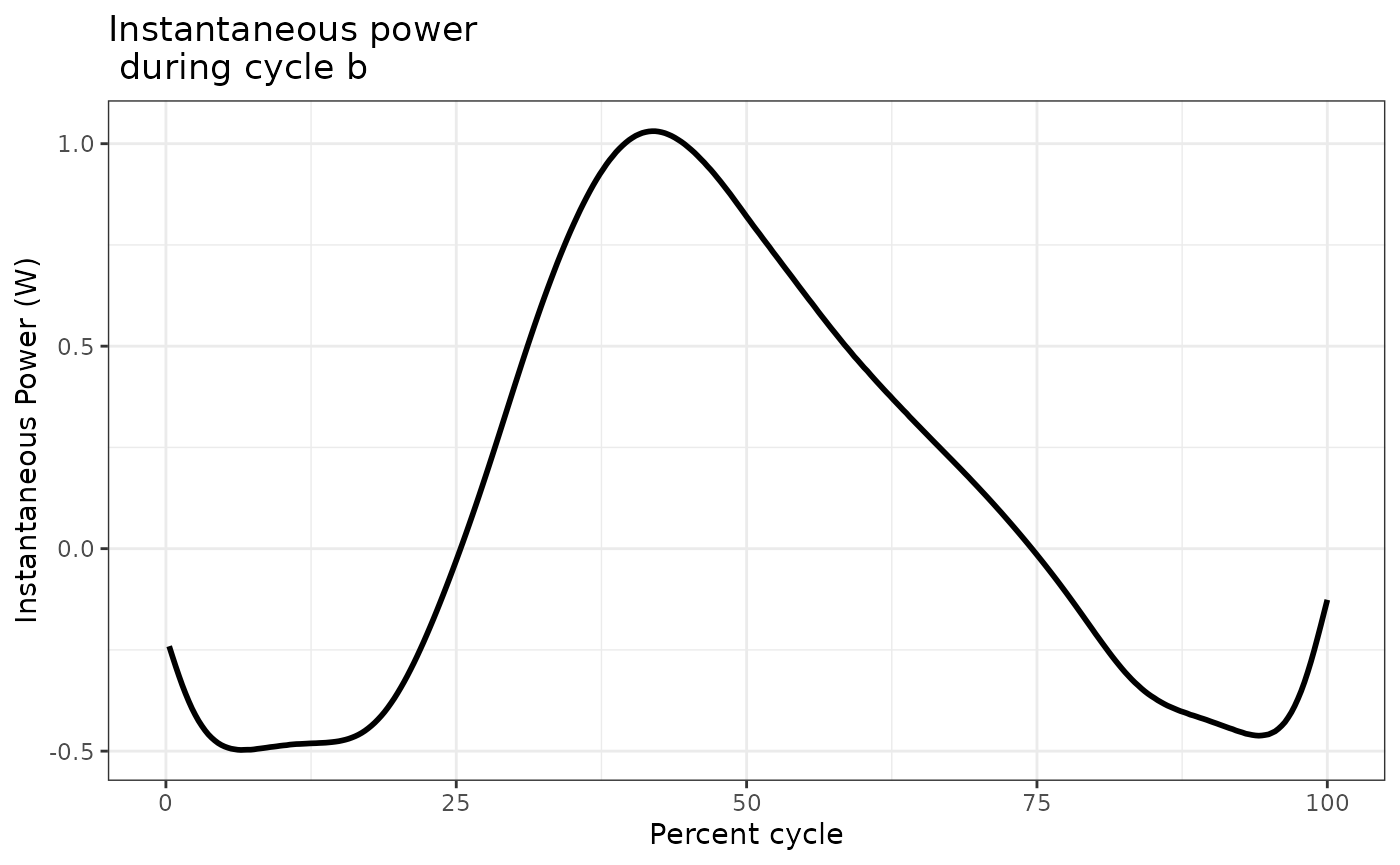
Setting simpilfy = TRUE in the
analyze_workloop() function
If you simply want work and net power for each cycle without
retaining any of the time-course data, set simplify = TRUE
within analyze_workloop().
workloop_analyzed_simple <-
  workloop_selected %>%
  analyze_workloop(GR = 1, simplify = TRUE)

## Produces a simple data.frame:
workloop_analyzed_simple
#>   Cycle        Work  Net_Power
#> a     A 0.003007098 0.09085517
#> b     B 0.003282334 0.09870268
#> c     C 0.003601049 0.09812219
str(workloop_analyzed_simple)
#> 'data.frame':    3 obs. of  3 variables:
#>  $ Cycle    : chr  "A" "B" "C"
#>  $ Work     : num  0.00301 0.00328 0.0036
#>  $ Net_Power: num  0.0909 0.0987 0.0981
Here, work (in J) and net power (in W) are simply returned in a
data.frame that is organized by cycle. No other attributes
are stored.
More on cycle definitions in select_cycles()
As noted above, there are three options for cycle definitions within
select_cycles(), encoded as cycle_def. The
three options for how cycles can be defined are named based on the
starting (and ending) points of the cycle: L0-to-L0 (lo),
peak-to-peak (p2p), and trough-to-trough
(t2t).
We highly recommend that you plot your Position data after using
select_cycles(). The pracma::findpeaks()
function work for most data (especially sine waves), but it is
conceivable that small, local ‘peaks’ may be misinterpreted as a cycle’s
true minimum or maximum.
We also note that edge cases (i.e. the first cycle or the final cycle) may also be subject to issues in which the cycles are not super well defined via an automated algorithm.
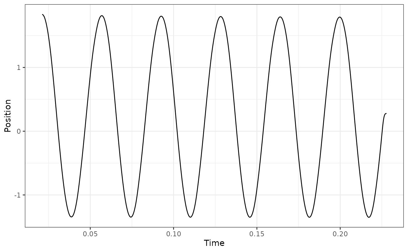
Below, we will plot a couple case examples to show what we generally
expect. We recommend plotting your data in a similar fashion to verify
that select_cycles() is behaving in the way you expect.
## Select cycles 4:6 using lo
workloop_dat %>%
  select_cycles(cycle_def="lo", keep_cycles = 4:6) %>%
  ggplot(aes(x = Time, y = Position)) +
  geom_line() +
  theme_bw()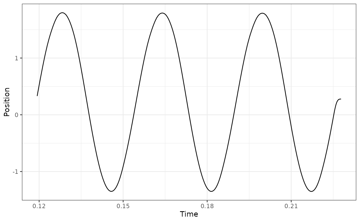
## Select cycles 4:6 using p2p
workloop_dat %>%
  select_cycles(cycle_def="p2p", keep_cycles = 4:6) %>%
  ggplot(aes(x = Time, y = Position)) +
  geom_line() +
  theme_bw()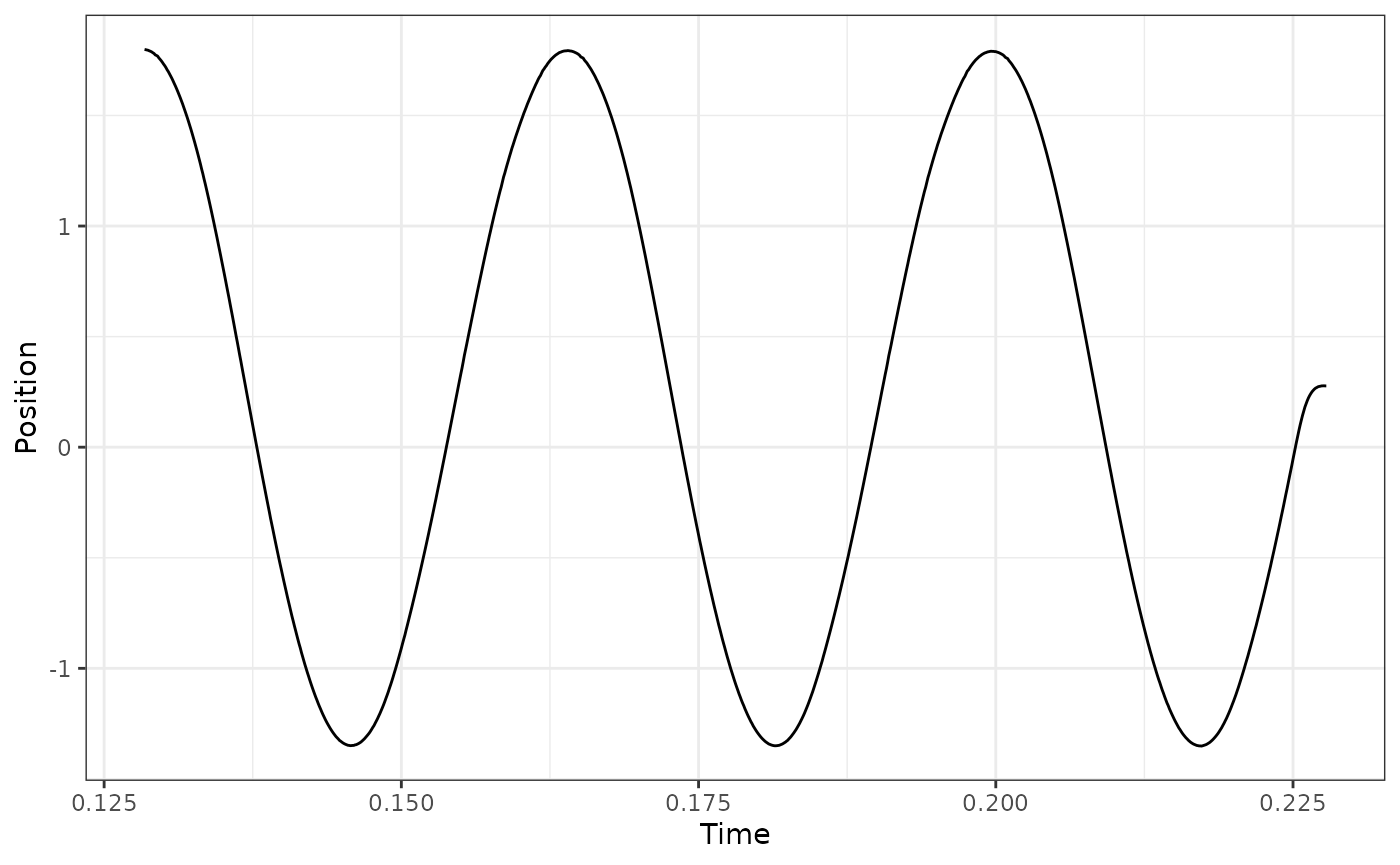
## here we see that via 'p2p' the final cycle is ill-defined because the return
## to L0 is considered a cycle. Using a p2p definition, what we actually want is
## to use cycles 3:5 to get the final 3 full cycles:
workloop_dat %>%
  select_cycles(cycle_def="p2p", keep_cycles = 3:5) %>%
  ggplot(aes(x = Time, y = Position)) +
  geom_line() +
  theme_bw()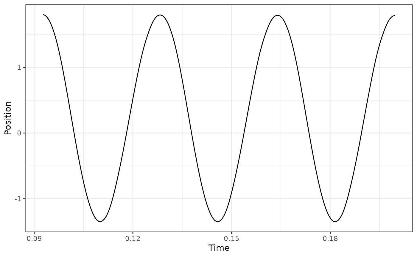
## this difficulty in defining cycles may be more apparent by first plotting the
## cycles 1:6, e.g.
workloop_dat %>%
  select_cycles(cycle_def="p2p", keep_cycles = 1:6) %>%
  ggplot(aes(x = Time, y = Position)) +
  geom_line() +
  theme_bw()