The very first thing to do is read the documentation on our README page. Make sure you have the package properly installed, and that your personal AIMS Data Platform API Key has been downloaded.
As per the installation instructions, we strongly suggest that you
hide your API Key permanently in your .Renviron file and
set the object my_api_key to NULL in the chunk
below. You can read more about why that is important here.
# set my_api_key to NULL after successfully placing it in .Renviron
my_api_key <- NULL
We now load dataaimsr:
How this package works
dataaimsr contains two sets of monitoring data collected
by AIMS—the Australian Institute of
Marine Science—since the 1980’s: the Weather Station
dataset which contains encompasses data for different parameters
(e.g. Air Temperature, Air Pressure, Chlorophyll, and many others); and
the Sea Water
Temperature Loggers dataset which contains records of (you guessed
it!) sea water temperature at different sites and water depths.
The datasets are very large, and as such they are not locally stored. They are instead downloaded via the API and unique DOI identifier (just hover over the data links above to see the actual DOI codes). The datasets are structured by sites, series and parameters. A series is a continuing time-series, i.e. a collection of deployments measuring the same parameter (e.g. Air Temperature, Air Pressure, Chlorophyll) at the same subsite. So, for a given site and parameter, there might exist multiple subsites and therefore series, in which case they are most likely distinguishable by depth.
For the Sea Water Temperature Loggers dataset, series is synonymous with the variable called subsite. For the Weather Station dataset, it is the combination of subsite and parameter.
This vignette gives an overview of how one would go about discovering the overall information contained in the datasets. For dataset-specific vignettes, see our other vignette pages.
Discover a dataset
The AIMS Data Platform API points to the full metadata of each dataset. We are currently working on ways to facilitate the visualisation of both datasets and their multiple features directly through the R package. At the moment though it is only possible to visualise summary information for the Sea Water Temperature Loggers dataset. A similar feature for the Weather Station dataset will be implemented in the near future (likely early 2021)—so for now, please refer to the online metadata to discover from where (and when) you can download data.
Data summary
The first step would be to visualise the dataset. Let’s do this by
mapping all available sites for the Sea Water Temperature Loggers
dataset using the main function called aims_data:
sdata <- aims_data(target = "temp_loggers", api_key = my_api_key,
                   summary = "summary-by-series")
head(sdata)
#>   site_id                    site subsite_id    subsite series_id     series         parameter
#> 1       1 Agincourt Reef Number 3       2687     AG3FL1      2687     AG3FL1 Water Temperature
#> 2       1 Agincourt Reef Number 3      14276  AG3SL1old     14276  AG3SL1old Water Temperature
#> 3       3           Cleveland Bay       3007 CLEVAWSSL1      3007 CLEVAWSSL1 Water Temperature
#> 4       3           Cleveland Bay       3069 CLEVAWSFL1      3069 CLEVAWSFL1 Water Temperature
#> 5       4             Davies Reef       2629     DAVFL1      2629     DAVFL1 Water Temperature
#> 6       4             Davies Reef       2630     DAVSL1      2630     DAVSL1 Water Temperature
#>   parameter_id time_coverage_start time_coverage_end      lat      lon depth uncal_obs cal_obs
#> 1            1          1996-03-30        2008-12-11 -15.9903 145.8212     0     23130  110480
#> 2            1          1996-03-30        2011-07-21 -15.9905 145.8213     5    114450  216794
#> 3            1          2004-05-13        2008-05-03 -19.1557 146.8813     7     11951   53231
#> 4            1          2005-09-15        2005-12-22 -19.1557 146.8813     1         0    4656
#> 5            1          1997-08-26        2019-06-10 -18.8065 147.6688     1    437544  566585
#> 6            1          1996-05-02        2022-03-05 -18.8060 147.6686     8    512106  638452
#>   qc_obs
#> 1 110480
#> 2 216794
#> 3  53231
#> 4   4656
#> 5 566585
#> 6 638397
The summary argument here is key. It should be either
"summary-by-series" or "summary-by-deployment"
when the user wants an overview of the available data. Again, this is
currently implemented for the Sea Water Temperature Loggers dataset
only. The output of aims_data is a data.frame
of class aimsdf.
Notice that sdata contains a lot of information, most of
which is related to site / series / parameter ID. Each row corresponds
to a unique series, and a certain site may contain multiple series; in
such cases, series generally differ from one another by depth. The
columns time_coverage_start and
time_coverage_end are probably one of the most valuable
pieces of information. They provide the user with the window of data
collection for a particular series, which is probably crucial to decide
whether that particular series is of relevance to the specific question
in hand.
Also note that there are three columns containing the total number of
observations in a series: uncal_obs, cal_obs
and qc_obs, which respectively stand for uncalibrated,
calibrated, and quality-controlled observations. Calibrated and
quality-controlled are generally the same. Instruments are routinely
calibrated (mostly once a year) in a temperature-controlled water bath
and corrections applied to the data. After calibration, all data records
are quality controlled based on the following tests: 1) clip to in-water
only data, using deployment’s metadata, 2) impossible value check: data
outside a fixed temperature range (14˚C – 40˚C) is flagged as bad data,
3) spike test: individual extreme values are flagged as probably bad and
4) Excessive gradient test: pairs of data that present a sudden change
in the slope are flagged as probably bad. If any data record fails at
least one of the tests, a QC flag equal to 2 is returned, otherwise, the
QC flag is set to 1.
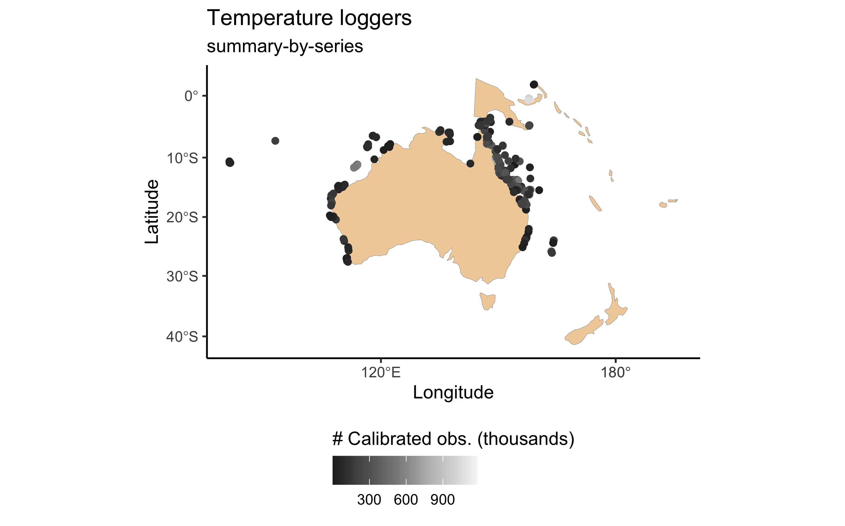
aimsdf objects can be plotted using the
plot function. For summary-by-... data such as
sdata, plot will always generate a map with
the points around Australia and associated regions, coloured by the
number of calibrated observations:
plot(sdata, ptype = "map")
Filter values
In the case of the Weather Station dataset, knowing what sites are
out there is a bit tricky. However, currently we have a convenience
function called aims_filter_values which allows one to
query what sites, series and parameters are available for both
datasets:
head(aims_filter_values("weather", filter_name = "series"))
#>   series_id                                                                 series
#> 1    104918        Myrmidon Reef Weather Station Wind Speed (scalar avg b 10 min)
#> 2      3509               Lizard Island Relay Pole 2 Maximum Wind Speed 30 Minutes
#> 3    100686                            Saibai Island Weather Station Hail Duration
#> 4       266 Orpheus Island Relay Pole 3 Wind Direction (Vector Average 30 Minutes)
#> 5      2639 Hardy Reef Weather Station Wind Direction (Vector Standard 10 Minutes)
#> 6     10243                           Raine Island Weather Station Air Temperature
The downside is that one cannot know what time window is available for each one of those, nor how they are nested (i.e. series / parameter / site). In a way though the series name generally gives that information anyway (see code output above). If knowing the available observation window is absolutely crucial, then as mentioned above the user should refer to the online metadata.
Download slices of datasets
Now that we know how to explore the datasets and what data is out there, we finish this vignette by showing an example of how one would go about downloading actual monitoring data.
We say slices of datasets because AIMS monitoring datasets are of very high temporal resolution and if one tries to download the entire thing it might take hours. Generally that is why we download slices of data at a time, and for that we need filters (see below).
On the other hand, if all we are interested in are aggregated values
(daily means), then we can set summary = "daily" in
aims_data in combination with a list of
filters to download more concise datasets. So far,
aggregated data is only available for the Sea Water Temperature Loggers
dataset.
Data filters
Filters are the last important information the user needs to know to
master the navigation and download of AIMS monitoring datasets. Each
dataset can filtered by attributes which can be exposed with the
function aims_expose_attributes:
aims_expose_attributes("weather")
#> $summary
#> [1] NA
#>
#> $filters
#>  [1] "site"      "subsite"   "series"    "series_id" "parameter" "size"      "min_lat"   "max_lat"
#>  [9] "min_lon"   "max_lon"   "from_date" "thru_date" "version"   "cursor"
aims_expose_attributes("temp_loggers")
#> $summary
#> [1] "summary-by-series"     "summary-by-deployment" "daily"
#>
#> $filters
#>  [1] "site"      "subsite"   "series"    "series_id" "parameter" "size"      "min_lat"   "max_lat"
#>  [9] "min_lon"   "max_lon"   "from_date" "thru_date" "version"   "cursor"
The help file (see ?aims_expose_attributes) contains the
details about what each filter targets. So, having an understanding of
the summaries and what filters are available provide the user with a
great head start.
Downloading the raw, high-resolution data is achieved using the same
aims_data function, however now we ignore the
summary argument, and instead implement filters. For
example, let’s say we want to download all the data collected at the Yongala for a
specific time window:
wdata_a <- aims_data("weather", api_key = my_api_key,
                     filters = list(site = "Yongala",
                                    from_date = "2018-01-01",
                                    thru_date = "2018-01-02"))
The returned aimsdf object in this case has attributes
which give us summary crucial information:
metadataa doi link containing the metadata record for the data seriescitationthe citation information for the particular datasetparametersan outputdata.frame
These can be directly extracted using the convenience functions
aims_metadata, aims_citation and
aims_parameters, e.g.:
aims_metadata(wdata_a)
#> [1] "Metadata record https://doi.org/10.25845/5c09bf93f315d"
This example data contains multiple parameters available for this
site at the specified time, and the actual measurements are either raw
or quality-controlled. For monitoring data (both aggregated or
non-aggregated, i.e. when summary = NA or
summary = "daily" in an aims_data call), we
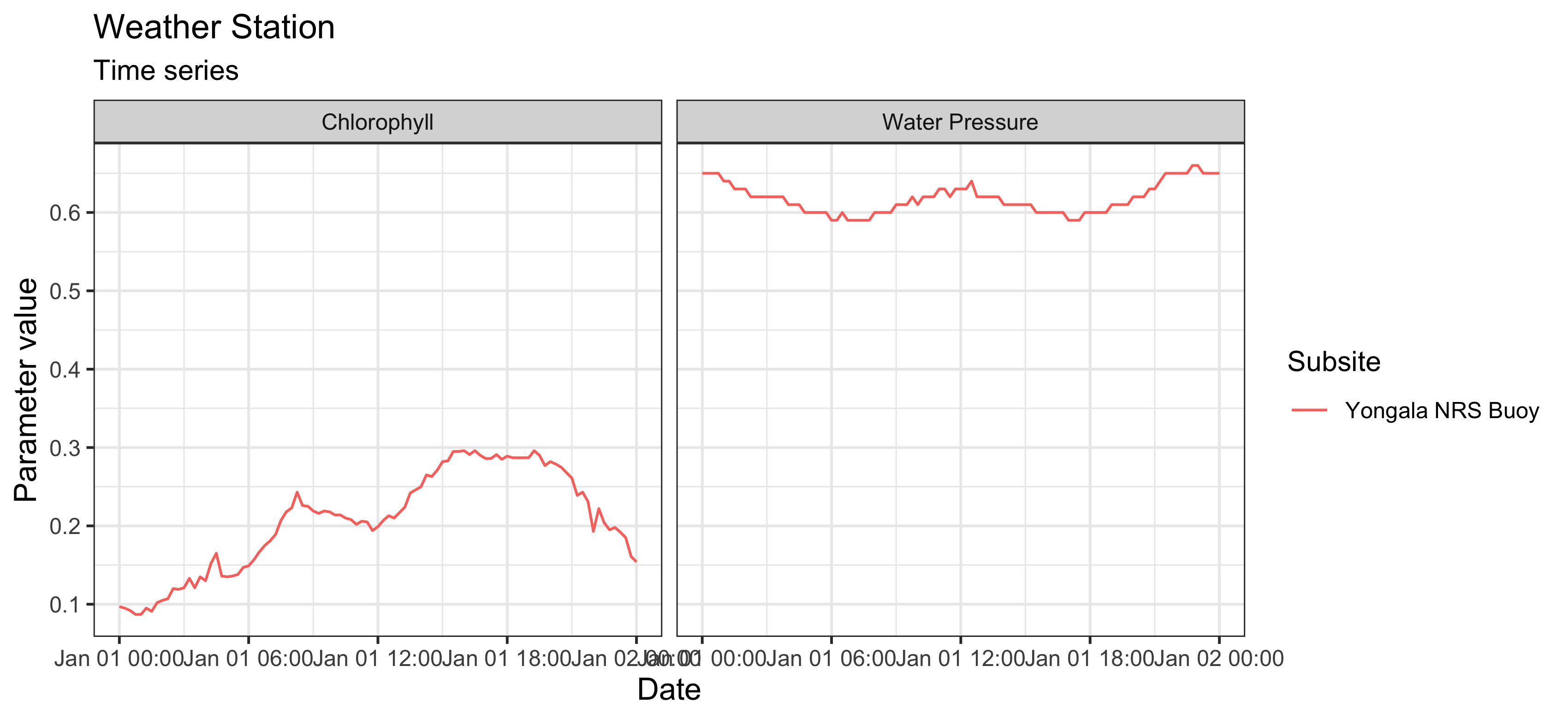
can either visualise the data as a time series broken down by parameter,
or a map showing the sites with some summary info. If the parameters are
not specified, then dataaimsr will plot a maximum of 4
parameters chosen at random for a time series plot. Alternatively the
user can specify which parameters are to be plotted.
# check parameters with aims_parameters(wdata_a)
plot(wdata_a, ptype = "time_series",
     pars = c("Water Pressure", "Chlorophyll"))
We can also refine even further by including a time window to download the data:
wdata_b <- aims_data("weather",
                     api_key = my_api_key,
                     filters = list(series_id = 64,
                                    from_date = "1991-10-18T06:00:00",
                                    thru_date = "1991-10-18T12:00:00"))
range(wdata_b$time)
#> [1] "1991-10-18 06:00:00 UTC" "1991-10-18 12:00:00 UTC"
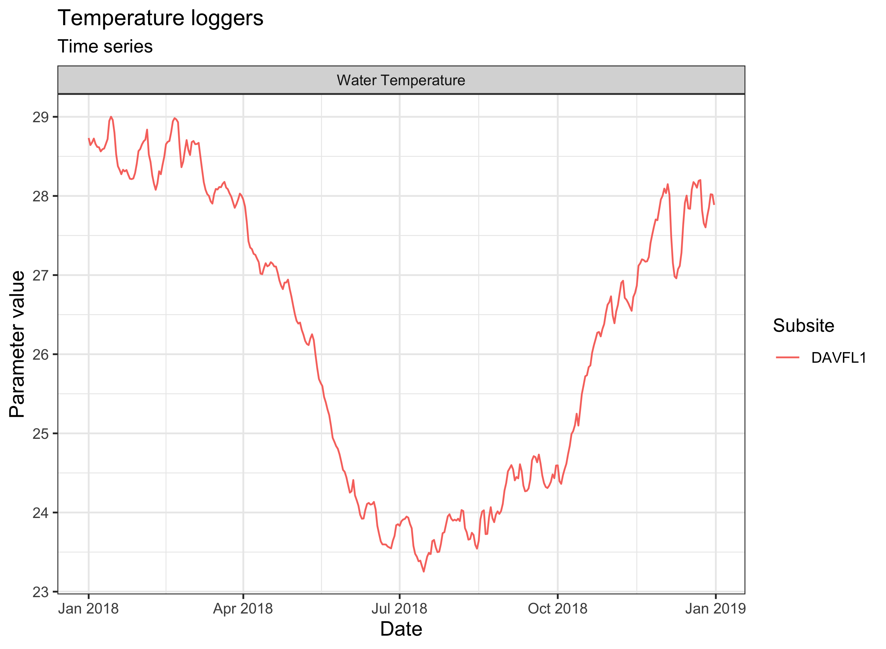
Or simply download and plot daily aggregated data:
sdata_c <- aims_data("temp_loggers", api_key = my_api_key, summary = "daily",
                     filters = list(series = "DAVFL1",
                                    from_date = "2018-01-01",
                                    thru_date = "2018-12-31"))
plot(sdata_c, ptype = "time_series", pars = c("Water Temperature"))
More info
See our other vignette pages for further dataset-specific explorations.
