Please check our intro vignette first to implement the installation requirements, and to learn the general approach to navigating the different datasets. This vignette assumes you have obtained an AIMS Data Platform API Key.
As per the installation instructions, we strongly suggest that you
hide your API Key permanently in your .Renviron file and
set the object my_api_key to NULL in the chunk
below. You can read more about why that is important here.
# set my_api_key to NULL after successfully placing it in .Renviron
my_api_key <- NULL
Let’s start by loading the packages needed for this vignette:
Discovering the dataset
The Sea Water Temperature Loggers dataset is less extensive than the AIMS Weather Station dataset because it comprises one single “parameter”—water temperature—that is measured at multiple sites. Not all sites have the same temporal coverage; some loggers are still actively collecting data, others have been discontinued. So the key distinctive variables in this instance are the “site”, and the “series”. A “series” represents a continuing time-series, i.e. a collection of deployments measuring the same parameter at the same subsite. Because there is only one parameter (water temperature), subsite and series are synonymous in the Sea Water Temperature Loggers dataset. So a series will comprise a continuing time-series at a specific site and depth.
Essentially, for the user who has limited knowledge about where the data are, and of what they are consisted, they would need to do some prior exploration to learn more about what can be downloaded. Suppose the goal is to download all time-series from a particular site. The general procedure would be:
- Examine documentation and establish query filters
- Perform data download using
aims_data - Create an exploratory time-series chart
For all datasets, a list of available filters can be retrieved with
the function aims_expose_attributes. Knowing the filters is
important because some time series are quite extensive, with parameters
being measured at very high frequency (e.g. every 5 minutes), so
downloading the dataset for an entire year or more my take quite some
time (it’s possible though if that is the true goal of the user).
Otherwise, the Sea Water Temperature Loggers dataset can be downloaded
at daily average aggregations, which can reduce the size of the download
by many fold.
aims_expose_attributes("temp_loggers")
#> $summary
#> [1] "summary-by-series"     "summary-by-deployment" "daily"
#>
#> $filters
#>  [1] "site"      "subsite"   "series"    "series_id" "parameter" "size"      "min_lat"   "max_lat"
#>  [9] "min_lon"   "max_lon"   "from_date" "thru_date" "version"   "cursor"
In the Sea Water
Temperature Loggers dataset, as demonstrated in our intro
vignette, we have a convenience summary argument which
facilitates learning more about what data is available. We can download
the summary information for all sites using the main function called
aims_data:
sdata <- aims_data("temp_loggers", api_key = my_api_key,
                   summary = "summary-by-series")
head(sdata)
#>   site_id                    site subsite_id    subsite series_id     series         parameter
#> 1       1 Agincourt Reef Number 3       2687     AG3FL1      2687     AG3FL1 Water Temperature
#> 2       1 Agincourt Reef Number 3      14276  AG3SL1old     14276  AG3SL1old Water Temperature
#> 3       3           Cleveland Bay       3007 CLEVAWSSL1      3007 CLEVAWSSL1 Water Temperature
#> 4       3           Cleveland Bay       3069 CLEVAWSFL1      3069 CLEVAWSFL1 Water Temperature
#> 5       4             Davies Reef       2629     DAVFL1      2629     DAVFL1 Water Temperature
#> 6       4             Davies Reef       2630     DAVSL1      2630     DAVSL1 Water Temperature
#>   parameter_id time_coverage_start time_coverage_end      lat      lon depth uncal_obs cal_obs
#> 1            1          1996-03-30        2008-12-11 -15.9903 145.8212     0     23130  110480
#> 2            1          1996-03-30        2011-07-21 -15.9905 145.8213     5    114450  216794
#> 3            1          2004-05-13        2008-05-03 -19.1557 146.8813     7     11951   53231
#> 4            1          2005-09-15        2005-12-22 -19.1557 146.8813     1         0    4656
#> 5            1          1997-08-26        2019-06-10 -18.8065 147.6688     1    437544  566585
#> 6            1          1996-05-02        2022-03-05 -18.8060 147.6686     8    512106  638452
#>   qc_obs
#> 1 110480
#> 2 216794
#> 3  53231
#> 4   4656
#> 5 566585
#> 6 638397
summary should be set to either
summary-by-series or summary-by-deployment
when the user wants an overview of the available data.
ddata <- aims_data("temp_loggers", api_key = my_api_key,
                   summary = "summary-by-deployment")
head(ddata)
#>   deployment_id serial_num site_id          site subsite_id subsite series_id  series
#> 1         39691   SU-11424       4   Davies Reef       2630  DAVSL1      2630  DAVSL1
#> 2        494247     203112     923  Geoffrey Bay      14475 GBMMPFL     14475 GBMMPFL
#> 3          3319 SST-905242     865 Hayman Island       2644  HAYSL1      2644  HAYSL1
#> 4        471410   10048402    3181    Enderby Is      14056 ENDERBY     14056 ENDERBY
#> 5         15923   SU-10088     986   Pine Island       3080 PINESL1      3080 PINESL1
#> 6        479464     355088     896    Turner Cay       2664  TURSL1      2664  TURSL1
#>           parameter parameter_id time_coverage_start time_coverage_end      lat      lon depth
#> 1 Water Temperature            1          2012-11-10        2013-05-21 -18.8060 147.6686   8.3
#> 2 Water Temperature            1          2020-04-06        2021-02-22 -19.1548 146.8685   2.0
#> 3 Water Temperature            1          1999-06-03        2000-05-15 -20.0572 148.8997   9.0
#> 4 Water Temperature            1          2015-05-24        2016-02-06 -20.5689 116.5550    NA
#> 5 Water Temperature            1          2011-09-28        2012-02-13 -20.3780 148.8884   6.6
#> 6 Water Temperature            1          2014-08-27        2017-01-25 -21.7031 152.5605    NA
#>   uncal_obs cal_obs qc_obs
#> 1     27504   27504  27504
#> 2     92448   92448  92448
#> 3         0   16590  16590
#> 4     12292   12292  12292
#> 5     19728   19728  19728
#> 6    125856  125856 125856
Notice that sdata contains a lot of information, most of
which is related to site / series / parameter ID. Each row corresponds
to a unique series. The columns time_coverage_start and
time_coverage_end are probably one of the most valuable
pieces of information. They provide the user with the window of data
collection for a particular series, which is probably crucial to decide
whether that particular series is of relevance to the specific question
in hand.
The benefits to choosing a data series (or the numeric
equivalent, series_id) is that it comes from one location
and parameter type (here only water temperature), making the data easy
to plot. If we did not choose a data series from the Sea Water Temperature
Loggers dataset, we would have to specify additional arguments to
ensure the data is downloaded as expected.
Our values and filters might look like the following:
| Variable | Value | Description |
|---|---|---|
| series_id | 2687 | Found here, Agincourt Reef Number 3 |
| from_date | “2005-01-01” | We want to start charting on 1/1/2005 |
| thru_date | “2005-01-10” | We are plotting 10 days of data |
Query and Plot Dataset
After deciding on query parameters, we plug the series id into a
aims_data function:
agincourt <- aims_data("temp_loggers", api_key = my_api_key,
                       filters = list(series_id = 2687,
                                      from_date = "2005-01-01",
                                      thru_date = "2005-01-10"))
We can check that the query filters worked:
range(agincourt$time)
#> [1] "2005-01-01 UTC" "2005-01-10 UTC"
We can then visualise where in Australia that data is placed:
plot(agincourt, ptype = "map")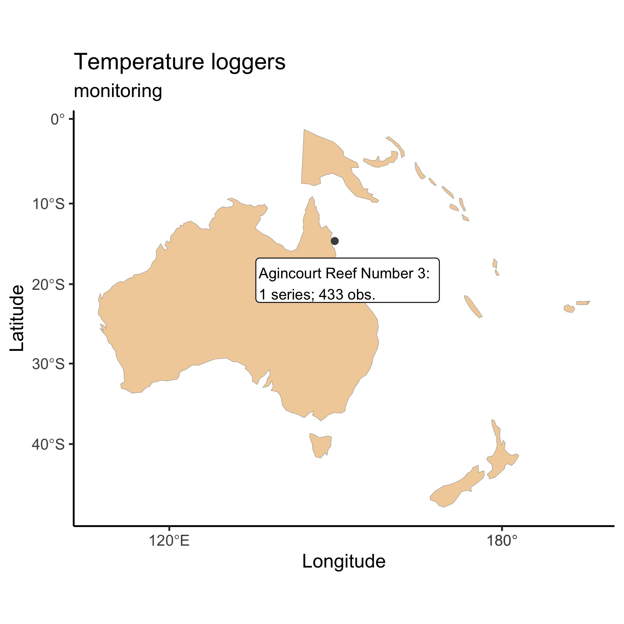
We can also visually compare multiple series at once. For instance, let’s compare the air temperature data from Davies Reef and Bramble Cay for the same period of time:
target_series <- c("Agincourt" = 2687, "Cleveland Bay" = 3007)
aims_data_per_series <- function(series_number, my_api_key, ...) {
  aims_data("temp_loggers", api_key = my_api_key,
            filters = list(series_id = series_number, ...))
}
results <- purrr::map(target_series, aims_data_per_series,
                      my_api_key = my_api_key,
                      from_date = "2005-01-01",
                      thru_date = "2005-01-10")
sst_data <- purrr::map_dfr(results, rbind)
plot(sst_data, ptype = "time_series")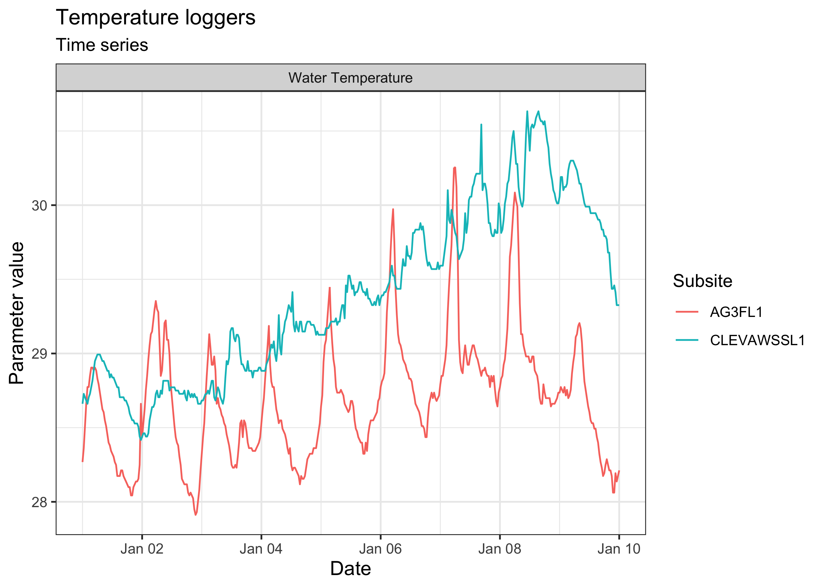
One could also download data for a particular time of day throughout
the year, e.g. for Davies Reef at 1 m of depth (series_id
is 2629):
days <- seq(as.Date("2005-01-01"), as.Date("2005-12-31"), by = "month")
out <- numeric(length = length(days))
for (i in seq_along(days)) {
  hour_in <- paste0(days[i], "T06:00:00")
  hour_out <- paste0(days[i], "T12:00:00")
  df <- aims_data("temp_loggers", api_key = my_api_key,
                  filters = list(series_id = 2629, from_date = hour_in,
                                 thru_date = hour_out))
  out[i] <- mean(df$qc_val)
}

ggplot(data = data.frame(date = days, temps = out)) +
  geom_line(mapping = aes(x = date, y = temps)) +
  labs(x = "Date",
       y = "Water temperature (˚C)",
       title = "Davies Reef @ 1 m (2005)",
       subtitle = "mean 6 A.M. – 12 P.M.") +
  theme_bw() +
  theme(axis.title.x = element_text(size = 12),
        axis.title.y = element_text(size = 12),
        legend.position = "bottom")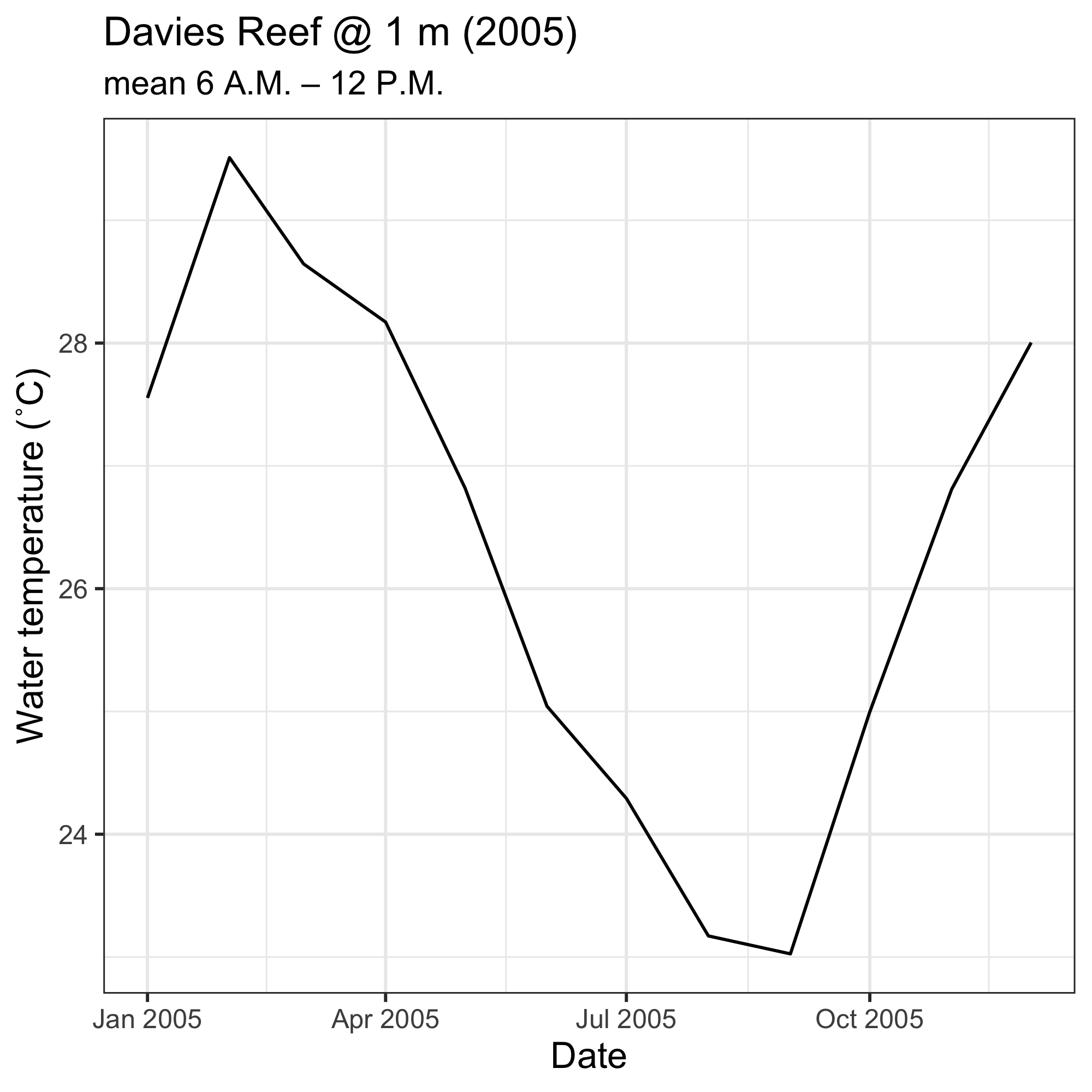
Or simply plot the daily aggregated averages:
df <- aims_data("temp_loggers", api_key = my_api_key, summary = "daily",
                filters = list(series_id = 2629, from_date = "2005-01-01",
                               thru_date = "2005-12-31"))
plot(df, ptype = "time_series", pars = c("Water Temperature"))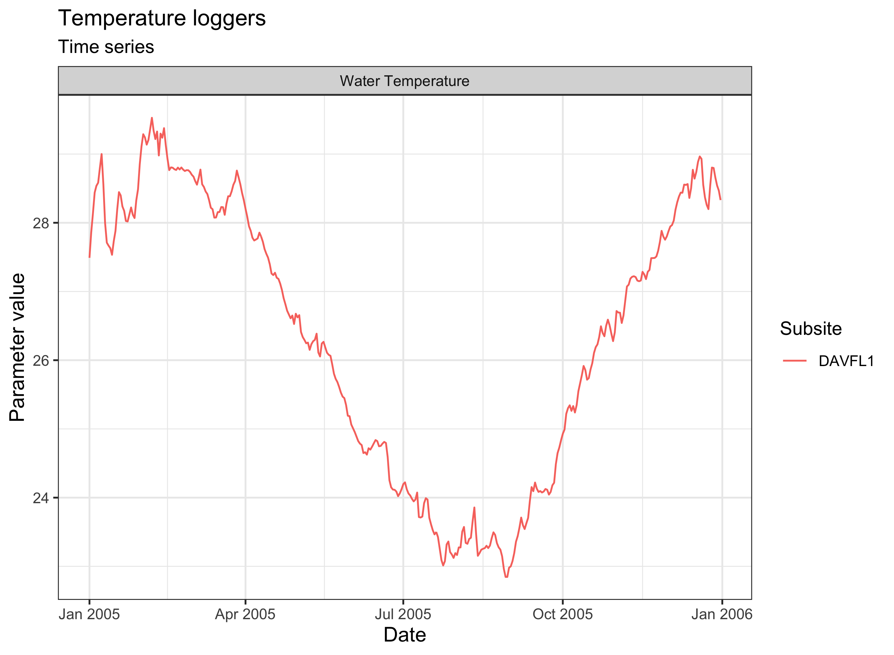
Bibliography
purrr::map_chr(results, aims_citation) %>%
  unlist %>%
  unname
#> [1] "Australian Institute of Marine Science (AIMS). 2017, AIMS Sea Temperature Observing System (AIMS Temperature Logger Program), Time period:2005-01-01 to 2005-01-10. https://doi.org/10.25845/5b4eb0f9bb848, accessed 06 Jul 2022."
#> [2] "Australian Institute of Marine Science (AIMS). 2017, AIMS Sea Temperature Observing System (AIMS Temperature Logger Program), Time period:2005-01-01 to 2005-01-10. https://doi.org/10.25845/5b4eb0f9bb848, accessed 06 Jul 2022."