Introduction to the Nomis API
nomisr is for accessing Nomis data with R. The Nomis API
is free to access without registration, and contains up-to-date official
statistics, including data from the Census, the Labour Force Survey, DWP
benefit statistics and other economic and demographic data. Nomis is
maintained on behalf of the Office for National Statistics by the
University of Durham.
There is a lot of data available through Nomis, and there are some limits to the amount of data that can be retrieved within a certain period of time, although those are not published. For more details, see the full API documentation from Nomis.
Nomis data is based around administrative and statistical geographies, and a particular geography should be specified when downloading data.
nomisr is designed around a pipeline of three key
functions: nomis_data_info(),
nomis_get_metadata() and nomis_get_data(). The
nomis_overview(), nomis_content_type() and
nomis_search() functions can assist with this.
Querying data availability
The nomis_data_info() function is focused on the
structure and coverage of the available datasets.
Use the nomis_data_info() function without any
parameters to get a tibble with metadata for all available datasets:
x <- nomis_data_info()
head(x)
nomis_data_info() can also be used to query metadata
from a specific dataset, using its ID. The example below uses the
“LC4408EW - Tenure by number of persons per bedroom in household by
household type” dataset from the 2011 census, which has the ID
“NM_893_1”.
library(nomisr)
y <- nomis_data_info("NM_893_1")

tibble::glimpse(y)
## Rows: 1
## Columns: 12
## $ agencyid <chr> "NOMIS"
## $ id <chr> "NM_893_1"
## $ uri <chr> "Nm-893d1"
## $ version <dbl> 1
## $ annotations.annotation <list> [<data.frame[14 x 2]>]
## $ components.attribute <list> [<data.frame[7 x 4]>]
## $ components.dimension <list> [<data.frame[6 x 3]>]
## $ components.primarymeasure.conceptref <chr> "OBS_VALUE"
## $ components.timedimension.codelist <chr> "CL_893_1_TIME"
## $ components.timedimension.conceptref <chr> "TIME"
## $ name.value <chr> "LC4408EW - Tenure by number of p…
## $ name.lang <chr> "en"When a tibble with metadata for all datasets or a specific dataset is
returned, three of the columns, annotations.annotation,
components.attribute and components.dimension,
are list-columns of data frames. annotations.annotation
contains metadata on the dataset, including units and current status.
components.attribute contains more detailed status
metadata. components.dimension contains the grouping and
summary variables available in the dataset, which vary between different
datasets.
The example below shows how to access data stored in list columns
returned from the Nomis API. In the case of requests for metadata from a
single dataset, the three columns are all lists with a length of 1. If
requesting all dataset information with nomis_data_info(),
each row is a list of length 1. Each list contains a data.frame, of
varrying dimensions depending on the column and dataset. You can unnest
individual list-columns to display their data in the same row as data
from the rest of the tibble. Due to the differing lengths of the
list-columns returned by nomis_data_info(), only one
list-column can be unnested at a time.
library(dplyr, warn.conflicts = F)

y$annotations.annotation %>% class()

y$annotations.annotation %>% length()

y$annotations.annotation[[1]] %>% class()

y %>% pull(annotations.annotation) %>% class()

y %>% pull(annotations.annotation) %>% .[[1]] %>% class()

y %>% pull(annotations.annotation) %>% purrr::pluck() %>% class()

## Unnesting list columns
y %>% tidyr::unnest(annotations.annotation) %>% glimpse()
Searching for data
nomisr also contains the nomis_search()
function to search for datasets on particular topics.
nomis_search() can be used to search in one or more of
dataset names, descriptions, keywords, content type and units. If using
multiple parameters, nomis_search() will return information
on all datasets that match one or more parameters. Character vectors of
strings can be used in searches, and likewise
nomis_search() will return information on datasets that
match one or more queries. The * is used as a wildcard symbol.
nomis_search() returns metadata in the same format as
nomis_data_info(), including using list-columns. The
nomis_content_type() function can assist in identifying
content type IDs for nomis_search().
Other ways to access metadata
nomis_overview() returns a tibble with a generalised
overview of a given dataset.
q <- nomis_overview("NM_1650_1")

q %>% tidyr::unnest(name) %>% glimpse()
nomis_overview() has a select parameter
that can be used to select only particular elements of the overview to
return.
Querying data variables
Vast amounts of data are available through Nomis and so to avoid
overwhelming the API, it is good practice to query what concepts are
available, using nomis_get_metadata(). While the other
metadata functions can return concept metadata,
nomis_get_metadata() provides greater flexibility and
specificity over the returned metadata than
nomis_overview() and nomis_data_info().
The example below queries some of the metadata available through the API for the “LC4408EW - Tenure bynumber of persons per bedroom in household by household type” dataset.
Getting concepts
If provided with just a dataset ID, nomis_get_metadata()
will return the concepts available for the given dataset.
a <- nomis_get_metadata(id = "NM_893_1")Concept Values
If provided with a concept name it returns the available values for
that concept. However, in some cases, espescially with the geography
concept, there are multiple options available, which Nomis labels types.
In that case nomis_get_metadata() returns the values of the
lowest indexed type available.
b <- nomis_get_metadata(id = "NM_893_1", concept = "GEOGRAPHY")We can now pass a generic “type” string to the type
parameter in nomis_get_metadata(), which returns all
available geography types for dataset “NM_893_1”.
c <- nomis_get_metadata(id = "NM_893_1", concept = "geography", type = "type")Passing a specific type to the type parameter, in this
case “TYPE460” for all post-2010 parliamentary constituencies, returns a
tibble with geographic codes for those specific constituencies, which
can be used to filter queries.
d <- nomis_get_metadata(id = "NM_893_1",
                        concept = "geography", type = "TYPE460")
The vast majority (98% as of February 2018) of Nomis datasets include a geographic variable.
Downloading data
Using the information above, we can now query the latest data on bedroom occupancy per household type in different NHS clinical commissioning groups.
z <- nomis_get_data(id = "NM_893_1", time = "latest", geography = "TYPE266")We can also query bedroom occupancy per household type in the Manchester, Gorton and Manchester, Withington parliamentary constituencies.
x <- nomis_get_data(id = "NM_893_1", time = "latest",
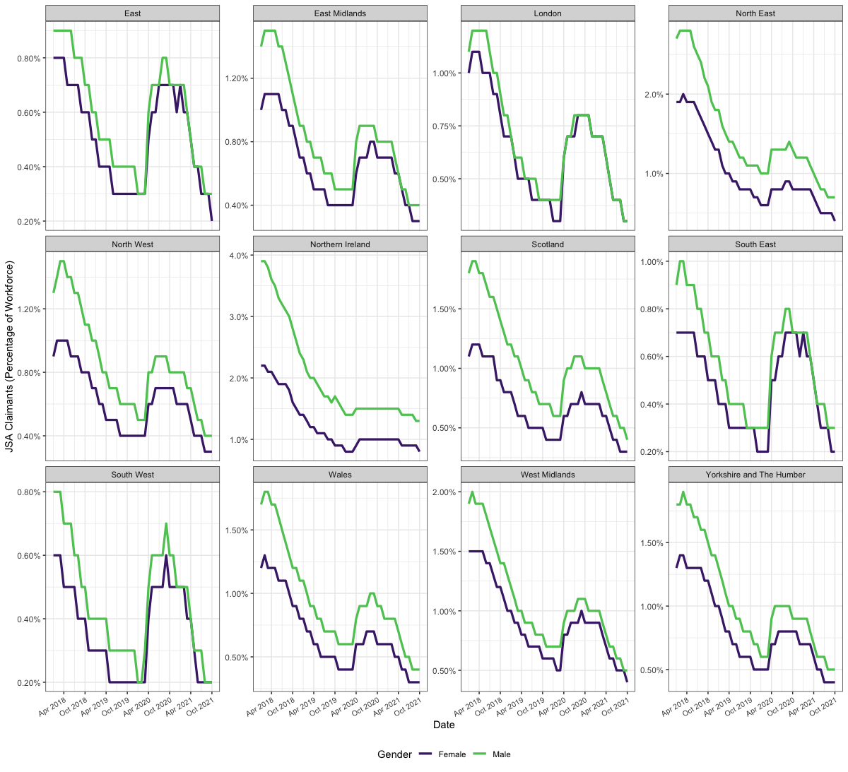
geography = c("1929380119", "1929380120"))nomisr also allows for time series queries. The example
below shows how to retrieve the percentage of the workforce claiming
Jobseekers Allowance from January 2015 to January 2020, inclusive, for
each region of the UK, divided by male and female claimants, with an
accompanying graph.
library(ggplot2)
library(dplyr)
library(nomisr)

jsa <- nomis_get_data(id = "NM_1_1", time = "2018-01-2021-10",
                      geography = "TYPE480", measures=20201,
                      sex=c(5,6), item = 1, tidy = TRUE)

jsa <- jsa %>%
  mutate(date = as.Date(paste0(date, "-01")),
         obs_value = obs_value/100)

theme_set(theme_bw())

p_jsa <- ggplot(jsa, aes(x = date, y = obs_value, colour = sex_name)) +
  geom_line(size = 1.15) +
  scale_colour_viridis_d(end = 0.75, begin = 0.1, name = "Gender") +
  scale_x_date(breaks = "6 months", date_labels = "%b %Y") +
  scale_y_continuous(labels = scales::percent) +
  theme(axis.text.x = element_text(angle = 30, hjust = 1, size = 8),
        legend.position = "bottom") +
  labs(x = "Date", y= "JSA Claimants (Percentage of Workforce)") +
  facet_wrap(~geography_name, scales = "free_y")

p_jsa