rOPTRAM: Three Trapezoid Fitting Methods

Introduction

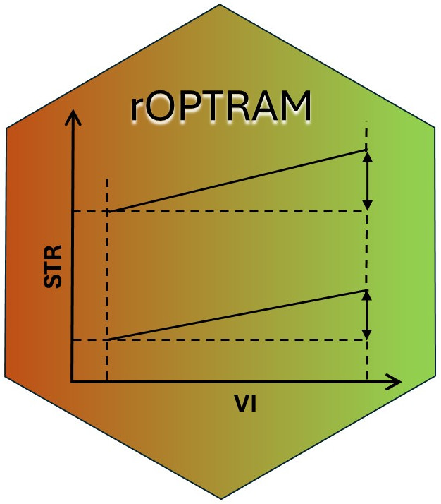
The algorithm for finding trapezoid wet and dry edges works as follows:

After acquiring a time series of Sentinel-2 images over the study area, both vegetation index (i.e. NDVI or SAVI), and SWIR Transformed Reflectance (STR) rasters are prepared. Pixel values of both indices for all images are collected into a two column table (and plotted as a scatterplot). The vegetation axis (x-axis) is split into a large number of intervals (usually between 50 - 100). The width of each interval is configurable by the user through the vi_step parameter in optram_wetdry_coefficients(). Then for each interval the top and bottom 5% quantiles of STR values are determined. These point values - VI and STR - are considered to create the fitted wet and dry trapezoid edges.

Three fitting methods are available in {rOPTRAM} to prepare the trapezoid wet and dry edges. For detailed background, see: Ma, Johansen, and McCabe (2022). Users can choose between a

• linear OLS fitted line
• exponential fit
• second order polynomial

All fitting methods are derived using the lm function in the R {stats} package.

The linear OLS fit follows: \[STR = i + s \cdot VI\] The exponential fit uses the equation: \[STR = i \cdot e^{(s \cdot VI)}\] where STR is the fitted STR value, \(i\), and \(s\) are the exponential regression intercept, and coefficient and \(VI\) is the vegetation index value.

The polynomial fit uses:

\[ STR = \alpha + \beta1 \cdot VI + \beta2 \cdot VI^2\]

The fitting method is chosen by setting the trapezoid_method option using the optram_options() function.

Examples

remotes::install_github("ropensci/rOPTRAM")
library("rOPTRAM")
library("CDSE")
library("jsonlite")

Prepare data.frame of pixel values

from_date <- "2022-05-01"
to_date <- "2023-04-30"
output_dir <- tempdir()
aoi <- sf::st_read(system.file("extdata",
                            "lachish.gpkg", package = "rOPTRAM"))
optram_options("veg_index", "NDVI")

s2_file_list <- optram_acquire_s2(aoi,
                            from_date, to_date,
                            output_dir = output_dir)
STR_list <- list.files(file.path(output_dir, "STR"),
                      pattern = ".tif$", full.names = TRUE)
VI_list <- list.files(file.path(output_dir, "NDVI"),
                      pattern = ".tif$", full.names = TRUE)
full_df <- optram_ndvi_str(STR_list, VI_list,
                           output_dir = output_dir)

Show Linear trapezoid plot

meth <- "linear"
optram_options("trapezoid_method", meth)
#> [1] "edge_points = TRUE"
#> [1] "feature_col = ID"
#> [1] "max_cloud = 12"
#> [1] "max_tbl_size = 1e+06"
#> [1] "period = full"
#> [1] "plot_colors = no"
#> [1] "remote = scihub"
#> [1] "rm.hi.str = FALSE"
#> [1] "rm.low.vi = FALSE"
#> [1] "SWIR_band = 11"
#> [1] "trapezoid_method = linear"
#> [1] "veg_index = NDVI"
#> [1] "vi_step = 0.005"

rmse <- optram_wetdry_coefficients(full_df,
                                   output_dir = output_dir)
edges_df <- read.csv(file.path(output_dir, "trapezoid_edges_lin.csv"))
pl <- plot_vi_str_cloud(full_df,  edges_df = edges_df,
                        edge_points = TRUE)

Trapezoid scatterplot

pl <- pl + ggplot2::ggtitle("Lachish area trapezoid plot",
                            subtitle = paste(meth, "fitted"))
ggplot2::ggsave(file.path(output_dir, paste0("trapezoid_lachish_",
                                             meth, ".png")),
                width = 18, height = 12, units = "cm")

Show Exponential fitted trapezoid plot

meth <- "exponential"
optram_options("trapezoid_method", meth)
#> [1] "edge_points = TRUE"
#> [1] "feature_col = ID"
#> [1] "max_cloud = 12"
#> [1] "max_tbl_size = 1e+06"
#> [1] "period = full"
#> [1] "plot_colors = no"
#> [1] "remote = scihub"
#> [1] "rm.hi.str = FALSE"
#> [1] "rm.low.vi = FALSE"
#> [1] "SWIR_band = 11"
#> [1] "trapezoid_method = exponential"
#> [1] "veg_index = NDVI"
#> [1] "vi_step = 0.005"

coeffs <- optram_wetdry_coefficients(full_df,
                                     output_dir = output_dir)
edges_df <- read.csv(file.path(output_dir, "trapezoid_edges_exp.csv"))
pl <- plot_vi_str_cloud(full_df,  edges_df = edges_df,
                        edge_points = TRUE)

Exponential fit trapezoid scatterplot

pl <- pl + ggplot2::ggtitle("Lachish area trapezoid plot",
                            subtitle = paste(meth, "fitted"))
ggplot2::ggsave(file.path(output_dir, paste0("trapezoid_lachish_",
                                            meth, ".png")),
                width = 18, height = 12, units = "cm")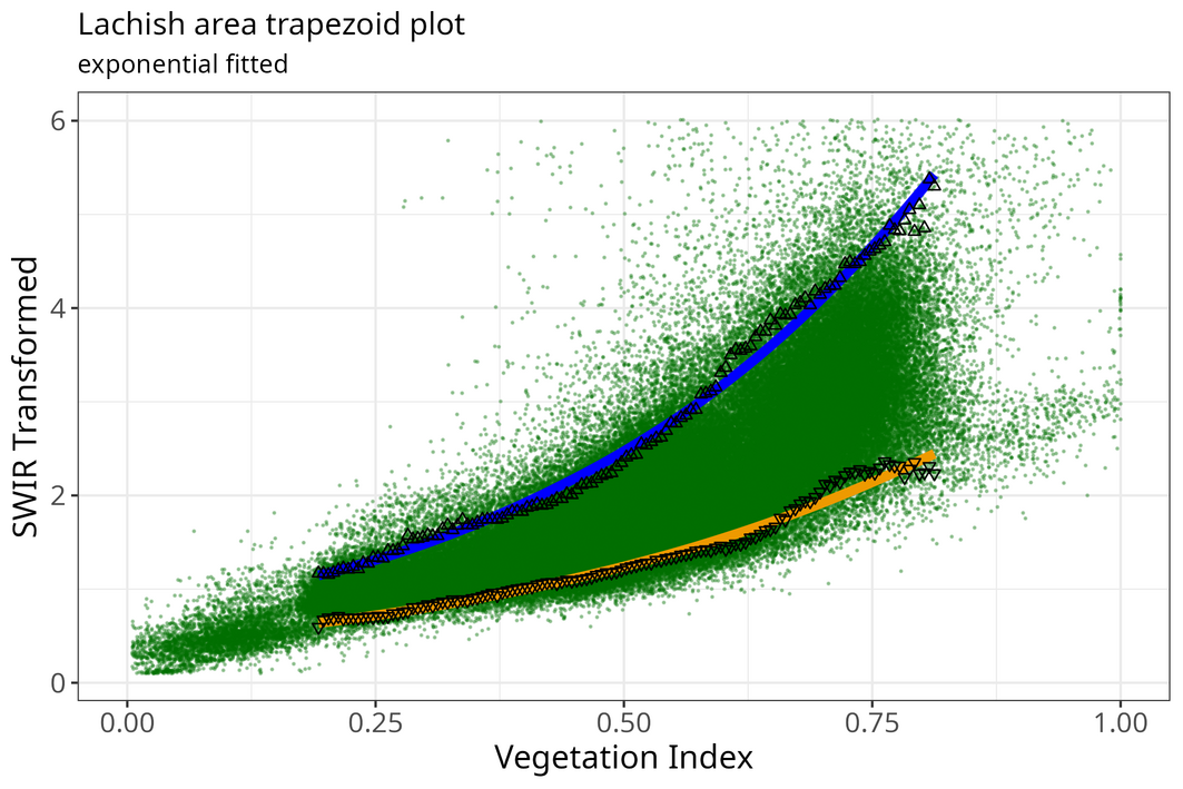

Show Polynomial fitted trapezoid plot

meth <- "polynomial"
optram_options("trapezoid_method", meth)
#> [1] "edge_points = TRUE"
#> [1] "feature_col = ID"
#> [1] "max_cloud = 12"
#> [1] "max_tbl_size = 1e+06"
#> [1] "period = full"
#> [1] "plot_colors = no"
#> [1] "remote = scihub"
#> [1] "rm.hi.str = FALSE"
#> [1] "rm.low.vi = FALSE"
#> [1] "SWIR_band = 11"
#> [1] "trapezoid_method = polynomial"
#> [1] "veg_index = NDVI"
#> [1] "vi_step = 0.005"

coeffs <- optram_wetdry_coefficients(full_df,
                                     output_dir = output_dir)
edges_df <- read.csv(file.path(output_dir, "trapezoid_edges_poly.csv"))
pl <- plot_vi_str_cloud(full_df,  edges_df = edges_df,
                        edge_points = TRUE)

Polynomial fit trapezoid scatterplot

pl <- pl + ggplot2::ggtitle("Lachish area trapezoid plot",
                            subtitle = paste(meth, "fitted"))
ggplot2::ggsave(file.path(output_dir, paste0("trapezoid_lachish_",
                                             meth, ".png")),
                width = 18, height = 12, units = "cm")

Ma, Chunfeng, Kasper Johansen, and Matthew F. McCabe. 2022. “Combining Sentinel-2 Data with an Optical-Trapezoid Approach to Infer Within-Field Soil Moisture Variability and Monitor Agricultural Production Stages.” Agricultural Water Management 274 (December): 107942. https://doi.org/10.1016/j.agwat.2022.107942.