Get started with rmangal

Context

The Mangal project

The Mangal project aims at archiving published ecological networks and at easing their retrieval. To do so, Mangal:

uses a data specification for ecological networks (described in Poisot et al. 2016);
archives ecological networks in a PostgreSQL database;
provides:

a data explorer to visualize and download data available;
a RESTful Application Programming Interface (API);
a client library for Julia: Mangal.jl;
a client of this API for R: the rmangal package described below.

Currently, 175 datasets are included in the database representing over 1300 ecological networks. In 2016, the first paper describing the project was published and introduced the first release of rmangal (Poisot et al. 2016). Since then, the structure of the database has been improved (new fields have been added), several ecological networks have been added and the API entirely rewritten. Consequently, the first release of the rmangal is obsolete (and archived) and we introduce rmangal v2.0 in this vignette. This vignette was reviewed on November 2022, when version 2.2 was released.

Data structure

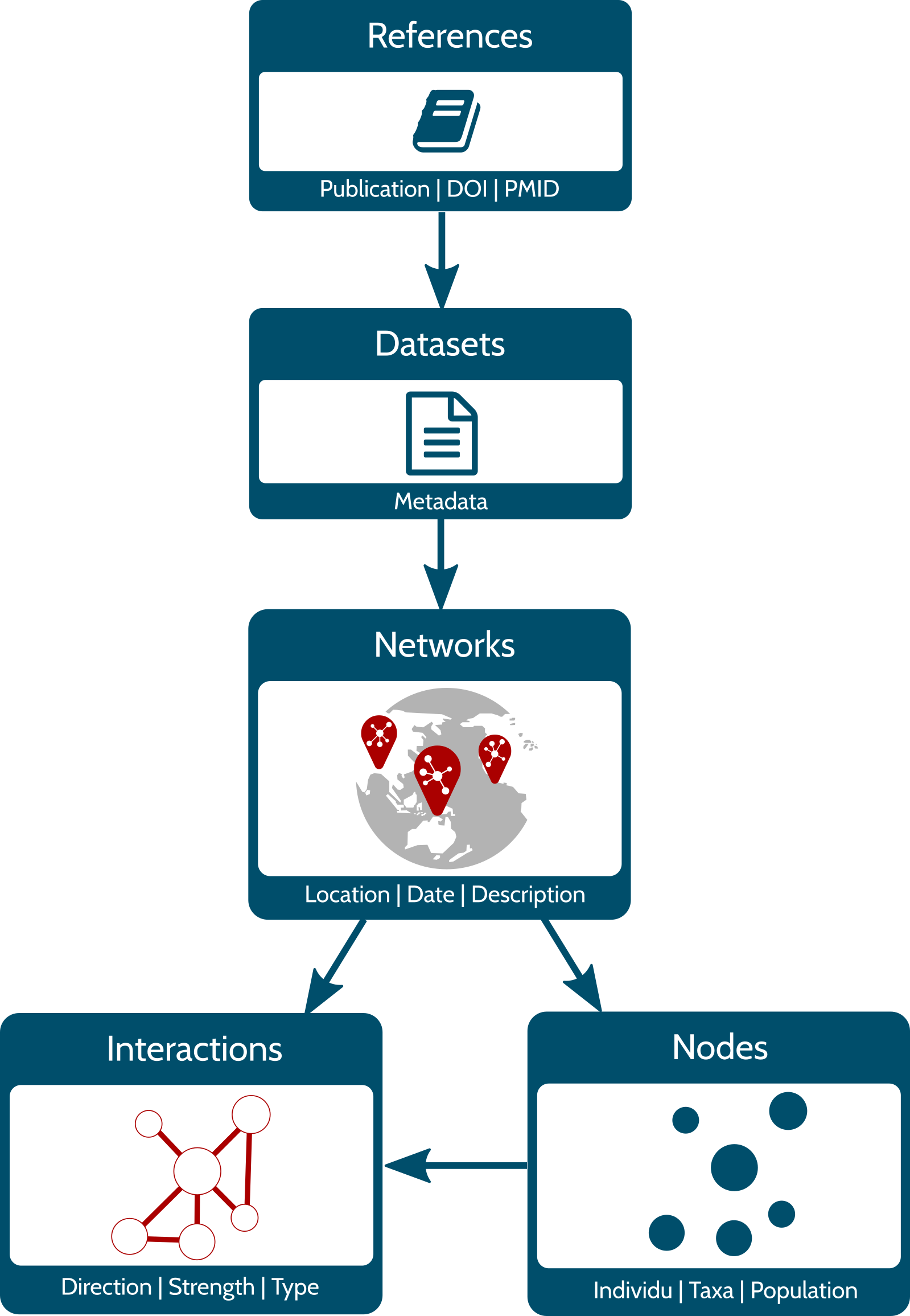
Diagram of the structure of the Mangal database

The diagram on the left side represents the structure of the Mangal database. All references included in Mangal correspond to a specific publication that includes one or several dataset(s). This dataset is basically a collection of ecological networks whose nodes and interactions (edges) are stored in separate tables. Below, we briefly describe the content of each table.

References – Information pertaining to a reference (scientific article, book, online website, etc.) characterizing an original collection of ecological networks. URLs of data and publication sources are included as well as persistent identifiers (when available) such as digital object identifiers (DOIs). This allows users to retrieve more details about original publications using appropriate R packages such as crossref.

Datasets – Metadata of the datasets attached to a reference. It includes a general description of the networks.

Networks – Metadata of the networks attached to a dataset. It provides the sampling location, date and specific description of the network.

Nodes – Information on the population, taxa or individual in the network. Each node has the original taxon name documented and a taxonomic backbone provided by all services embedded in taxize (Chamberlain et al. 2019).

Interactions – Information on the interaction type (e.g. mutualism, predation, etc.), the strength, and the direction of the interaction between two nodes.

Authentication

So far, the rmangal package provides methods to get access to the data store. Data requests (performed via rmangal_request() or rmangal_request_singleton()) do not require any authentication.

A bearer authentication strategy using ORCID credentials (as a third-party services) has been implemented on all POST, DELETE, PUT API operations to allow the user to add and delete new ecological to the database. These features are not currently included in the rmangal package, but remain under consideration for future major releases.

How to use rmangal

Overall approach

In order to efficiently retrieve networks from the database, rmangal includes 7 search functions querying the 5 tables described above as well as a table dedicated to the taxonomy backbone.

search_references(): search in the reference table, for instance the user can look for a specific doi;
search_datasets(): search among datasets using a keyword;
search_networks() and search_networks_sf(): search networks based on a keyword or a geographical area;
search_interactions(): list all networks containing a specific interaction type;
search_nodes(): identify nodes based on nodes information;
search_taxonomy(): identify nodes based on taxonomic names and unique identifiers.

All of these functions return specific class objects with the information needed to retrieve the corresponding set of ecological networks with get_collection(). Hence, the user can easily retrieve data in two steps:

networks <- search_*(query = "your query") |> get_collection()

If there is only one network to be retrieved, get_collection() returns a mgNetwork object, otherwise it returns an object of class mgNetworksCollection which is a collection (a list) of mgNetwork objects. Below, we exemplify how to use the search functions, how to get a collection of networks and how to use other packages to carry out specific analyses.

Requests can be cached (rmangal leverages httr2::req_cache()) either by setting the argument cache to TRUE or by providing a path that points to the desired cache directory. Using cache the basic workflow becomes:

networks <- search_*(query = "your query", cache = TRUE) |> get_collection()

Search functions

In rmangal, every function queries a specific table and allows only one query at a time (see section Batch analysis to learn how to perform more than one query). All the functions offer two ways to query the corresponding table:

a keyword: in this case, the entries returned are the partial or full keyword match of any strings contained in the table;
a custom query: in this case, entries returned are exact matches.

We start by loading rmangal as well as tibble (enhanced data frames).

library(rmangal)
library(tibble)

Search and list available datasets

Let’s assume we are looking for ecological networks including species living in lagoons. If we have no idea about any existing data set, the best starting point is then to query the dataset table with lagoon as a keyword:

lagoon <- search_datasets(query = "lagoon")
class(lagoon)
#> [1] "tbl_df"           "tbl"              "data.frame"       "mgSearchDatasets"
lagoon
#> # A tibble: 2 × 10
#>      id name        description                                     public created_at             updated_at ref_id user_id networks references
#>   <int> <chr>       <chr>                                           <lgl>  <chr>                  <chr>       <int>   <int> <list>   <list>    
#> 1    22 zetina_2003 Dietary matrix of the Huizache–Caimanero lagoon TRUE   2019-02-23T17:04:32.0… 2019-02-2…     22       3 <df>     <df>      
#> 2    52 yanez_1978  Food web of the Guerrero lagoon                 TRUE   2019-02-24T23:42:52.0… 2019-02-2…     53       3 <df>     <df>

If the Mangal reference identifiers of this dataset is known, the following query can be used:

lagoon_zetina <- search_datasets(list(ref_id = 22))
lagoon_zetina
#> # A tibble: 1 × 10
#>      id name        description                                     public created_at             updated_at ref_id user_id networks references
#>   <int> <chr>       <chr>                                           <lgl>  <chr>                  <chr>       <int>   <int> <list>   <list>    
#> 1    22 zetina_2003 Dietary matrix of the Huizache–Caimanero lagoon TRUE   2019-02-23T17:04:32.0… 2019-02-2…     22       3 <df>     <df>

Note that if an empty character is passed, i.e. "", all entries are returned.

all_datasets <- search_datasets("")
head(all_datasets)
#> # A tibble: 6 × 10
#>      id name                  description                                       public created_at updated_at ref_id user_id networks references
#>   <int> <chr>                 <chr>                                             <lgl>  <chr>      <chr>       <int>   <int> <list>   <list>    
#> 1     2 howking_1968          Insect activity recorded on flower at Lake Hazen… TRUE   2019-02-2… 2019-02-2…      2       2 <df>     <df>      
#> 2     7 lundgren_olesen_2005  Pollnator activity recorded on flowers, Uummanna… TRUE   2019-02-2… 2019-02-2…      7       2 <df>     <df>      
#> 3     9 elberling_olesen_1999 Flower-visiting insect at Mt. Latnjatjarro, nort… TRUE   2019-02-2… 2019-02-2…      9       2 <df>     <df>      
#> 4    14 johnston_1956         Predation by short-eared owls on a salicornia sa… TRUE   2019-02-2… 2019-02-2…     14       3 <df>     <df>      
#> 5    15 havens_1992           Pelagic communities of small lakes and ponds of … TRUE   2019-02-2… 2019-02-2…     15       3 <df>     <df>      
#> 6    16 kemp_1977             Food web for the Crystal River estuary            TRUE   2019-02-2… 2019-02-2…     16       3 <df>     <df>
length(all_datasets)
#> [1] 10

As shown in the diagram above, a dataset comes from a specific reference and search_references() queries the reference table directly. A handy argument of this function is doi as it allows to pass a Digital Object Identifier and so to retrieve all datasets attached to a specific publication.

zetina_2003 <- search_references(doi = "10.1016/s0272-7714(02)00410-9")

Finding a specific network

We can also search by keywords across all networks.

insect_coll <- search_networks(query = "insect%")
head(insect_coll)
#>     id                               name                     date
#> 1   18    mosquin_martin_1967_19650731_18 1965-07-31T00:00:00.000Z
#> 2  909 elberling_olesen_1999_19940823_909 1994-08-23T00:00:00.000Z
#> 3  948             kato_1993_19910901_948 1991-09-01T00:00:00.000Z
#> 4 1460         cornaby_1974_19680208_1460 1968-02-08T00:00:00.000Z
#> 5 1461         cornaby_1974_19680229_1461 1968-02-29T00:00:00.000Z
#> 6 1471    jiron_cartin_1981_19770101_1471 1977-01-01T00:00:00.000Z
#>                                                                                                                                             description
#> 1                                Occurence of flower-visiting insect on plant species, two miles north of Bailey Point, Melville Island, N.W.T., Canada
#> 2                                                                                           Flower-visiting insect at Mt. Latnjatjarro, northern Sweden
#> 3 Flower and anthophilous insect interactions in the primary cool-temperate subalpine forests and meadows at Mt. Kushigata, Yamanashi Prefecture, Japan
#> 4                           The insect community of  a toad carrion in a tropical dry lowland forest at Finac La pacifica, Guanacaste Prov., Costa Rica
#> 5                             The insect community of  a toad carrion in a tropical wet lowland forest near Rincon de Osa, Puntarenas Prov., Costa Rica
#> 6                                              The insect community of a dog carcass in a premontane humid forest, University of Costa Rica, Costa Rica
#>   public all_interactions               created_at               updated_at dataset_id user_id geom_type  geom_lon geom_lat
#> 1   TRUE            FALSE 2019-02-22T18:38:37.491Z 2019-02-22T18:38:37.491Z          4       3     Point -114.9667       75
#> 2   TRUE            FALSE 2019-02-24T22:21:32.444Z 2019-02-24T22:21:32.444Z          9       2     Point      18.5    68.35
#> 3   TRUE            FALSE 2019-02-25T20:52:09.499Z 2019-02-25T20:52:09.499Z         66       2     Point  138.3833  35.5833
#> 4   TRUE            FALSE 2019-03-01T18:30:50.890Z 2019-03-01T18:30:50.890Z         91       4     Point -85.09443  10.4568
#> 5   TRUE            FALSE 2019-03-01T18:30:57.419Z 2019-03-01T18:30:57.419Z         91       4     Point -83.50833 8.534018
#> 6   TRUE            FALSE 2019-03-04T18:22:33.907Z 2019-03-04T18:22:33.907Z         99       4     Point -84.07651 9.933982

It is also possible to retrieve all networks based on interaction types involved:

comp_interac <- search_interactions(type = "competition")
# Number of competition interactions in mangal
nrow(comp_interac)
#> [1] 12

search_networks_sf() handles spatial queries: argument query_sf takes a sf object as input and returns all networks included in the spatial extent of this object. For instance, one can retrieve all networks found in North Carolina included in Mangal like so:

library(sf)
library(mapview)
area <- sf::st_read(system.file("shape/nc.shp", package="sf"))
#> Reading layer `nc' from data source `/usr/lib/R/site-library/sf/shape/nc.shp' using driver `ESRI Shapefile'
#> Simple feature collection with 100 features and 14 fields
#> Geometry type: MULTIPOLYGON
#> Dimension:     XY
#> Bounding box:  xmin: -84.32385 ymin: 33.88199 xmax: -75.45698 ymax: 36.58965
#> Geodetic CRS:  NAD27
in_NC <- search_networks_sf(area)

mapView(
  st_geometry(area), 
  color = "red", 
  legend = FALSE, 
  col.regions = "#FF000033"
  ) + mapView(in_NC, legend = FALSE)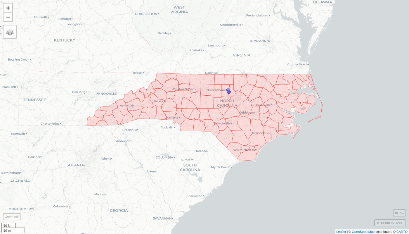

Map of the networks found in North Carolina

Search for a specific taxon

The user can easily identify networks including a specific taxonomic entity with search_taxonomy():

sr_ficus <- search_taxonomy("Ficus")

This function allows to search for a specific taxonomic entity with its validated name or unique identifiers, i.e. EOL, TSN, GBIF, COL, BOLD and NCBI IDs. Taxon names of the taxonomy table were validated with TNRS (see https://tnrs.biendata.org/) and/or GNR (see https://resolver.globalnames.org/). The taxon names in this table might not be the taxon name documented in the original publication. In order to identify relevant networks with the original name, use search_nodes().

The validation of taxon names was performed by an automated procedure using taxize (Chamberlain et al. 2019) and if there is any doubt, the original names recorded by authors should be regarded as the most reliable information. Please report any issue related to taxonomy at https://github.com/mangal-interactions/contribute/issues/new/choose.

head(search_taxonomy(tsn = 28749))
#>     id original_name node_level network_id taxonomy_id               created_at               updated_at taxonomy.id taxonomy.name
#> 1 2629  Acer negundo      taxon         19           2 2019-02-22T18:48:49.433Z 2019-02-22T18:48:49.433Z           2  Acer negundo
#>   taxonomy.ncbi taxonomy.tsn taxonomy.eol taxonomy.bold taxonomy.gbif                     taxonomy.col taxonomy.rank      taxonomy.created_at
#> 1          4023        28749       583069        100987       3189866 90203e29e2f59e5754167f89b9eba3cc       species 2019-02-21T21:17:12.585Z
#>        taxonomy.updated_at
#> 1 2019-06-14T15:20:36.273Z
head(search_taxonomy(eol = 583069))
#>     id original_name node_level network_id taxonomy_id               created_at               updated_at taxonomy.id taxonomy.name
#> 1 2629  Acer negundo      taxon         19           2 2019-02-22T18:48:49.433Z 2019-02-22T18:48:49.433Z           2  Acer negundo
#>   taxonomy.ncbi taxonomy.tsn taxonomy.eol taxonomy.bold taxonomy.gbif                     taxonomy.col taxonomy.rank      taxonomy.created_at
#> 1          4023        28749       583069        100987       3189866 90203e29e2f59e5754167f89b9eba3cc       species 2019-02-21T21:17:12.585Z
#>        taxonomy.updated_at
#> 1 2019-06-14T15:20:36.273Z

Note that in some cases, it may be necessary to locate a dataset using the original name provided in the publication; in such cases, the search_nodes() function should be used.

sr_ficus2 <- search_nodes("Ficus")

Get networks associated with a `search_*` object

Once the search performed, ecological networks are accessible from the object returned with get_collection():

nets_lagoons <- lagoon |> get_collection()
nets_in_NC <- in_NC |> get_collection()
nets_competition <- comp_interac |> get_collection()

nets_lagoons
class(nets_lagoons)
#> [1] "mgNetworksCollection"

Note that mgNetworksCollection objects are lists of mgNetwork object which are a list of five datasets reflecting the 5 tables presented in the diagram in the first section:

names(nets_lagoons[[1]])
#> [1] "network"      "nodes"        "interactions" "dataset"      "reference"
head(nets_lagoons[[1]]$network)
#>   network_id                    name                     date                                     description public all_interactions
#> 1         86 zetina_2003_20030101_86 2003-01-01T00:00:00.000Z Dietary matrix of the Huizache–Caimanero lagoon   TRUE            FALSE
#>                 created_at               updated_at dataset_id user_id geom_type  geom_lon geom_lat
#> 1 2019-02-23T17:04:34.046Z 2019-02-23T17:04:34.046Z         22       3     Point -106.1099 22.98531
head(nets_lagoons[[1]]$nodes)
#>   node_id original_name node_level network_id taxonomy_id               created_at               updated_at taxonomy.id taxonomy.name
#> 1    4904      Scianids      taxon         86        4363 2019-02-23T17:04:42.505Z 2019-02-23T17:04:42.505Z        4363    Sciaenidae
#> 2    4905       Elopids      taxon         86        4364 2019-02-23T17:04:42.571Z 2019-02-23T17:04:42.571Z        4364         Elops
#> 3    4906     Lutjanids      taxon         86        4365 2019-02-23T17:04:42.622Z 2019-02-23T17:04:42.622Z        4365    Lutjanidae
#> 4    4907     Carangids      taxon         86        4366 2019-02-23T17:04:42.672Z 2019-02-23T17:04:42.672Z        4366    Carangidae
#> 5    4908  Centropomids      taxon         86        4367 2019-02-23T17:04:42.728Z 2019-02-23T17:04:42.728Z        4367 Centropomidae
#> 6    4909        Ariids      taxon         86        4368 2019-02-23T17:04:42.786Z 2019-02-23T17:04:42.786Z        4368       Ariidae
#>   taxonomy.ncbi taxonomy.tsn taxonomy.eol taxonomy.bold taxonomy.gbif                     taxonomy.col taxonomy.rank      taxonomy.created_at
#> 1         30870       169237         5211          1856            NA 81a86c329909d507edb5c296906ef3f4        family 2019-02-23T17:04:35.620Z
#> 2          7927        28630     46561210          4061            NA 94532a14786adeb25bcec244a53aadc1         genus 2019-02-23T17:04:35.744Z
#> 3         30850       168845         5294          1858            NA 7150078b7dd31a5f7575240f1b76f834        family 2019-02-23T17:04:35.870Z
#> 4          8157       168584         5361          1851            NA 1ccc9e80931658b72d166c1764b687b5        family 2019-02-23T17:04:35.975Z
#> 5          8184       167642         5355           586            NA 529f1f934910702cb5334f8aa90cd22f        family 2019-02-23T17:04:36.102Z
#> 6         31017        43998         5115          1313            NA f60963ef9a967267b989ec22096edd3b        family 2019-02-23T17:04:36.207Z
#>        taxonomy.updated_at taxonomy
#> 1 2019-06-14T15:25:46.438Z       NA
#> 2 2019-06-14T15:25:46.492Z       NA
#> 3 2019-06-14T15:25:46.546Z       NA
#> 4 2019-06-14T15:25:46.600Z       NA
#> 5 2019-06-14T15:25:46.654Z       NA
#> 6 2019-06-14T15:25:46.708Z       NA
head(nets_lagoons[[1]]$interactions)
#>   interaction_id node_from node_to                     date direction      type method attr_id value geom public network_id
#> 1          48376      4912    4912 2003-01-01T00:00:00.000Z  directed predation     NA      12 0.026   NA   TRUE         86
#> 2          48377      4912    4914 2003-01-01T00:00:00.000Z  directed predation     NA      12 0.025   NA   TRUE         86
#> 3          48378      4912    4915 2003-01-01T00:00:00.000Z  directed predation     NA      12 0.003   NA   TRUE         86
#> 4          48379      4912    4918 2003-01-01T00:00:00.000Z  directed predation     NA      12 0.009   NA   TRUE         86
#> 5          48380      4912    4919 2003-01-01T00:00:00.000Z  directed predation     NA      12 0.009   NA   TRUE         86
#> 6          48381      4912    4920 2003-01-01T00:00:00.000Z  directed predation     NA      12 0.016   NA   TRUE         86
#>                 created_at               updated_at attribute.id attribute.name                                  attribute.description
#> 1 2019-02-23T17:05:45.061Z 2019-02-23T17:05:45.061Z           12 dietary matrix Proportions of the consumer diets made up by the prey.
#> 2 2019-02-23T17:05:45.131Z 2019-02-23T17:05:45.131Z           12 dietary matrix Proportions of the consumer diets made up by the prey.
#> 3 2019-02-23T17:05:45.193Z 2019-02-23T17:05:45.193Z           12 dietary matrix Proportions of the consumer diets made up by the prey.
#> 4 2019-02-23T17:05:45.247Z 2019-02-23T17:05:45.247Z           12 dietary matrix Proportions of the consumer diets made up by the prey.
#> 5 2019-02-23T17:05:45.309Z 2019-02-23T17:05:45.309Z           12 dietary matrix Proportions of the consumer diets made up by the prey.
#> 6 2019-02-23T17:05:45.367Z 2019-02-23T17:05:45.367Z           12 dietary matrix Proportions of the consumer diets made up by the prey.
#>   attribute.unit     attribute.created_at     attribute.updated_at
#> 1             NA 2019-02-23T17:04:25.350Z 2019-02-23T17:04:25.350Z
#> 2             NA 2019-02-23T17:04:25.350Z 2019-02-23T17:04:25.350Z
#> 3             NA 2019-02-23T17:04:25.350Z 2019-02-23T17:04:25.350Z
#> 4             NA 2019-02-23T17:04:25.350Z 2019-02-23T17:04:25.350Z
#> 5             NA 2019-02-23T17:04:25.350Z 2019-02-23T17:04:25.350Z
#> 6             NA 2019-02-23T17:04:25.350Z 2019-02-23T17:04:25.350Z
head(nets_lagoons[[1]]$dataset)
#>   dataset_id        name                                     description public               created_at               updated_at ref_id
#> 1         22 zetina_2003 Dietary matrix of the Huizache–Caimanero lagoon   TRUE 2019-02-23T17:04:32.017Z 2019-02-23T17:04:32.017Z     22
#>   user_id
#> 1       3
head(nets_lagoons[[1]]$reference)
#>   ref_id                           doi           first_author year jstor pmid
#> 1     22 10.1016/s0272-7714(02)00410-9 manuel j. zetina-rejon 2003    NA   NA
#>                                                                                                                                                                                                                                                                                                                                                                                                                                                                                                                     bibtex
#> 1 @article{Zetina_Rej_n_2003, doi = {10.1016/s0272-7714(02)00410-9}, url = {https://doi.org/10.1016%2Fs0272-7714%2802%2900410-9}, year = 2003, month = {aug}, publisher = {Elsevier {BV}}, volume = {57}, number = {5-6}, pages = {803--815}, author = {Manuel J. Zetina-Rejón and Francisco Arreguí-Sánchez and Ernesto A. Chávez}, title = {Trophic structure and flows of energy in the Huizache{\textendash}Caimanero lagoon complex on the Pacific coast of Mexico},journal = {Estuarine, Coastal and Shelf Science}}
#>                                             paper_url                 data_url               created_at               updated_at
#> 1 https://doi.org/10.1016%2Fs0272-7714%2802%2900410-9 https://globalwebdb.com/ 2019-02-23T17:04:28.307Z 2019-02-23T17:04:28.307Z

Integrated workflow with `rmangal`

Batch analysis

So far, the search functions of rmangal allow the user to perform only a single search at a time. The simplest way to do more than one search is to loop over a vector or a list of queries. Below we exemplify how to do so using lapply():

tsn <- c(837855, 169237)
mgn <- lapply(tsn, function(x) search_taxonomy(tsn = x)) |>
  lapply(get_collection) |>
  combine_mgNetworks()
mgn

Geolocate Mangal networks with `sf`

The function get_collection() has an argument as_sf than converts network metadata of mgNetwork objects to sf objects, which requires sf to be installed. This allows the user to easily track the location of the networks retrieved from Mangal.

# assuming sf and mapview are is loaded (as we did above)
mg_lag_sf <- search_datasets(query = 'lagoon') |> 
  get_collection(as_sf = TRUE)
class(mg_lag_sf[[1]]$network)
#> [1] "sf"         "data.frame"

# let's combine all these sf object into a single one
mapView(mg_lag_sf[[1]]$network) + mapView(mg_lag_sf[[2]]$network)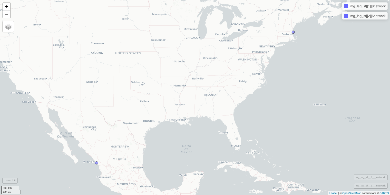

Map showing networks retrieved using the keywork ‘lagoon’

Taxonomic analysis

As Mangal includes taxonomic identifiers, rmangal can readily be combined with taxize (see taxize for more details about this package).

Network analysis with `igraph`

Once the data are retrieved and a mgNetwork or a mgNetworkCollection objects obtained, it is straightforward to convert it as a igraph (see the dedicated website) object and then to carry out network analysis:

library(igraph)
mg_lagoons <- search_datasets(query = 'lagoon')  |> get_collection()
# NB the line below returns a list of igraph objects
ig_lagoons <- as.igraph(mg_lagoons)
## Modularity analysis for the first network
modularity(ig_lagoons[[1]], membership(cluster_walktrap(ig_lagoons[[1]])))
#> [1] 0.05139834
## Degree values for all networks
lapply(ig_lagoons, degree)
#> [[1]]
#> 4904 4905 4906 4907 4908 4909 4910 4911 4912 4913 4914 4915 4916 4917 4918 4919 4920 4921 4922 4924 4925 4926 4927 4923 4929 4928 
#>   17   11   14   13   18   20   14   10   18   14   12   15    7   15   14   12   14   11   26    7   22   15   21   16    5   17 
#> 
#> [[2]]
#> 14395 14397 14398 14399 14400 14401 14402 14403 14404 14405 14406 14407 14408 14409 14411 14412 14413 14414 14415 14416 14417 14418 14419 
#>     9     5     7     7     5     5     5     4     5     5     5     3     2     4     7     7     5     9     9     5     1     3     5 
#> 14420 14422 14423 14424 14425 14426 14427 14396 14428 14410 14421 14429 
#>    11    17     4     3    11    11     5     9     5     3    11     2 
#> 
#> [[3]]
#> 14522 14523 14524 14525 14526 14527 14528 14530 14532 14537 14538 14539 14536 14531 14521 14529 14533 14534 14535 
#>     5     5     5     5     5     5     5     9     7     3     2     2     5     9     4     2     7     2     1 
#> 
#> [[4]]
#> 14430 14431 14432 14433 14434 14435 14436 14437 14438 14439 14440 14441 14442 14443 14444 14445 14446 14448 14449 14450 14451 14452 14453 
#>     9     9     5     3     5     8     9     8     9     7     9     3     1     9     8     5     5    12    22    25    23     3     3 
#> 14454 14455 14456 14458 14447 14457 
#>     3     3    11     8    12    11 
#> 
#> [[5]]
#> 14496 14497 14498 14499 14500 14501 14502 14503 14504 14505 14506 14507 14508 14511 14512 14513 14515 14516 14517 14518 14519 14520 14509 
#>     3     6     6     6     3     3     2     7     7     7     1     1    10     6     8     8     3     3     3     5     5     5     5 
#> 14510 14514 
#>     6     1 
#> 
#> [[6]]
#> 14459 14460 14461 14462 14463 14464 14465 14466 14467 14468 14469 14471 14472 14473 14474 14475 14476 14477 14478 14479 14480 14481 14482 
#>    12    12     1     6     6    15    15    15    15     6     4     9     9     9    13    13    13     2     2    14    14    12    17 
#> 14483 14485 14486 14487 14488 14491 14493 14494 14495 14492 14490 14470 14484 14489 
#>    17    17    12    12     7     7     2     2     2     7     7     4    17     3

Network manipulation and visualization with `tidygraph` and `ggraph`

The package tidygraph treats networks as two tidy tables (one for the edges and one for the nodes) that can be modified using the grammar of data manipulation developed in the tidyverse. Moreover, tidygraph wraps over most of the igraph functions so that the user can call a vast variety of algorithms to properly analysis networks. Fortunately, objects of class mgNetwork can readily be converted into tbl_graph objects which allows the user to benefit from all the tools included in tidygraph:

library(tidygraph)
# NB the line below would not work with a mgNetworksCollection (use lapply)
tg_lagoons <-  as_tbl_graph(mg_lagoons[[1]])  |>
  mutate(centrality_dg = centrality_degree(mode = 'in'))
tg_lagoons %E>% as_tibble()
#> # A tibble: 189 × 19
#>     from    to interaction_id date     direction type  method attr_id value public network_id created_at updated_at attribute.id attribute.name
#>    <int> <int>          <int> <chr>    <chr>     <chr> <lgl>    <int> <dbl> <lgl>       <int> <chr>      <chr>             <int> <chr>         
#>  1     9     9          48376 2003-01… directed  pred… NA          12 0.026 TRUE           86 2019-02-2… 2019-02-2…           12 dietary matrix
#>  2     9    11          48377 2003-01… directed  pred… NA          12 0.025 TRUE           86 2019-02-2… 2019-02-2…           12 dietary matrix
#>  3     9    12          48378 2003-01… directed  pred… NA          12 0.003 TRUE           86 2019-02-2… 2019-02-2…           12 dietary matrix
#>  4     9    15          48379 2003-01… directed  pred… NA          12 0.009 TRUE           86 2019-02-2… 2019-02-2…           12 dietary matrix
#>  5     9    16          48380 2003-01… directed  pred… NA          12 0.009 TRUE           86 2019-02-2… 2019-02-2…           12 dietary matrix
#>  6     9    17          48381 2003-01… directed  pred… NA          12 0.016 TRUE           86 2019-02-2… 2019-02-2…           12 dietary matrix
#>  7     9    18          48382 2003-01… directed  pred… NA          12 0.284 TRUE           86 2019-02-2… 2019-02-2…           12 dietary matrix
#>  8     9    19          48383 2003-01… directed  pred… NA          12 0.231 TRUE           86 2019-02-2… 2019-02-2…           12 dietary matrix
#>  9     9    21          48384 2003-01… directed  pred… NA          12 0.079 TRUE           86 2019-02-2… 2019-02-2…           12 dietary matrix
#> 10     9    22          48385 2003-01… directed  pred… NA          12 0.09  TRUE           86 2019-02-2… 2019-02-2…           12 dietary matrix
#> # ℹ 179 more rows
#> # ℹ 4 more variables: attribute.description <chr>, attribute.unit <lgl>, attribute.created_at <chr>, attribute.updated_at <chr>
tg_lagoons %N>% as_tibble() |>
  select(original_name, taxonomy.tsn, centrality_dg)
#> # A tibble: 26 × 3
#>    original_name  taxonomy.tsn centrality_dg
#>    <chr>                 <int>         <dbl>
#>  1 Scianids             169237             1
#>  2 Elopids               28630             0
#>  3 Lutjanids            168845             1
#>  4 Carangids            168584             2
#>  5 Centropomids         167642             2
#>  6 Ariids                43998             1
#>  7 Haemulids            169055             4
#>  8 Pleuronectoids       172859             3
#>  9 Callinectes           13951             6
#> 10 Belonoids            165546             4
#> # ℹ 16 more rows

Another strong advantage of tbl_graph objects is that there are the objects used by the package ggraph that that offers various functions (theme, geoms, etc.) to efficiently visualize networks:

library(ggraph)
ggraph(tg_lagoons, layout = "stress") +
  geom_edge_parallel(
    end_cap = circle(.5),
    start_cap = circle(.5),
    arrow = arrow(length = unit(1, 'mm'),
    type = 'closed')
  ) +
  geom_node_point(aes(colour = taxonomy.rank), size = 8) +
  theme_graph(background = "grey40", foreground = NA, text_colour = 'white')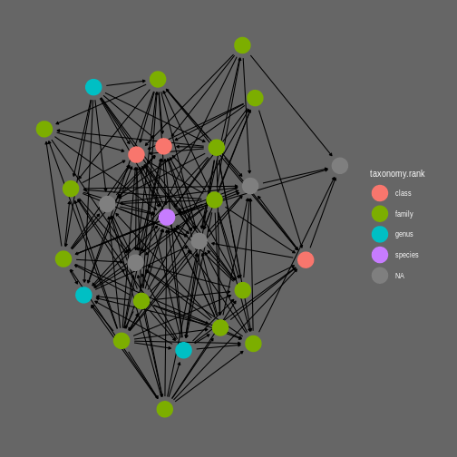

Example of network visualization with ggraph

Creating a list references for a set of networks

We can easily print the BibTeX of all publications involved in the networks collection.

search_datasets(query = 'lagoon') |>
  get_collection() |> 
  get_citation() |> 
  cat(sep = "\n\n")
#> @article{Zetina_Rej_n_2003, doi = {10.1016/s0272-7714(02)00410-9}, url = {https://doi.org/10.1016%2Fs0272-7714%2802%2900410-9}, year = 2003, month = {aug}, publisher = {Elsevier {BV}}, volume = {57}, number = {5-6}, pages = {803--815}, author = {Manuel J. Zetina-Rejón and Francisco Arreguí-Sánchez and Ernesto A. Chávez}, title = {Trophic structure and flows of energy in the Huizache{   extendash}Caimanero lagoon complex on the Pacific coast of Mexico},journal = {Estuarine, Coastal and Shelf Science}}
#> 
#> @article{Dexter_1947, doi = {10.2307/1948658}, url = {https://doi.org/10.2307%2F1948658}, year = 1947, month = {feb}, publisher = {Wiley}, volume = {17}, number = {3}, pages = {261--294}, author = {Ralph W. Dexter}, title = {The Marine Communities of a Tidal Inlet at Cape Ann, Massachusetts: A Study in Bio-Ecology}, journal = {Ecological Monographs}}

References

Chamberlain, Scott, Eduard Szoecs, Zachary Foster, Zebulun Arendsee, Carl Boettiger, Karthik Ram, Ignasi Bartomeus, et al. 2019. Taxize: Taxonomic Information from Around the Web. https://github.com/ropensci/taxize.

Poisot, Timothée, Benjamin Baiser, Jennifer A. Dunne, Sonia Kéfi, François Massol, Nicolas Mouquet, Tamara N. Romanuk, Daniel B. Stouffer, Spencer A. Wood, and Dominique Gravel. 2016. “Mangal - Making Ecological Network Analysis Simple.” Ecography 39 (4): 384–90.

Steve Vissault

Kevin Cazelles

2025-11-11

Context

The Mangal project

Data structure

Authentication

How to use rmangal

Overall approach

Search functions

Search and list available datasets

Finding a specific network

Search for a specific taxon

Get networks associated with a `search_*` object

Integrated workflow with `rmangal`

Batch analysis

Geolocate Mangal networks with `sf`

Taxonomic analysis

Network analysis with `igraph`

Network manipulation and visualization with `tidygraph` and `ggraph`

Creating a list references for a set of networks

References

About

Community

Resources

Get started with rmangal

Steve Vissault

Kevin Cazelles

2025-11-11

Context

The Mangal project

Data structure

Authentication

How to use rmangal

Overall approach

Search functions

Search and list available datasets

Finding a specific network

Search for a specific taxon

Get networks associated with a search_* object

Integrated workflow with rmangal

Batch analysis

Geolocate Mangal networks with sf

Taxonomic analysis

Network analysis with igraph

Network manipulation and visualization with tidygraph and ggraph

Creating a list references for a set of networks

References

Get networks associated with a `search_*` object

Integrated workflow with `rmangal`

Geolocate Mangal networks with `sf`

Network analysis with `igraph`

Network manipulation and visualization with `tidygraph` and `ggraph`