Introducing stats19
R Lovelace, M Morgan, L Hama and M Padgham
2026-01-29
Source:vignettes/stats19.Rmd
stats19.RmdIntroduction
stats19 enables access to and processing of Great Britain’s official road traffic casualty database, STATS19. A description of variables in the database can be found in a guidance provided by the UK’s Department for Transport (DfT). The datasets are collectively called STATS19 after the form used to report them, which can be found here. This vignette focuses on how to use the stats19 package to work with STATS19 data.
Note: The Department for Transport used to refer to ‘accidents’, but “crashes” may be a more appropriate term, as emphasised in the “crash not accident” arguments of road safety advocacy groups such as RoadPeace. We use the term collision only in reference to nomenclature within the data as provided.
The development version is hosted on GitHub and can be installed and loaded as follows:
# from CRAN
install.packages("stats19")
# you can install the latest development (discoraged) using:
remotes::install_github("ITSLeeds/stats19")Functions
The easiest way to get STATS19 data is with
get_stats19(). This function takes 2 main arguments,
year and type. The year can be any year
between 1979 and 202x where x is the current year minus one or two due
to the delay in publishing STATS19 statistics. The type can be one of
accidents, casualties and
vehicles, described below. get_stats19()
performs 3 jobs, corresponding to three main types of functions:
Download: A
dl_stats19()function acceptsyear,typeandfilenamearguments to make it easy to find the right file to download only.-
Read: STATS19 data is provided in a particular format that benefits from being read-in with pre-specified column types. This is taken care of with
read_*()functions providing access to the 3 main tables in STATS19 data:-
read_collisions()reads-in the crash data (which has one row per incident) -
read_casualties()reads-in the casualty data (which has one row per person injured or killed) -
read_vehicles()reads-in the vehicles table, which contains information on the vehicles involved in the crashes (and has one row per vehicle)
-
Format: There are corresponding
format_*()functions for each of theread_*()functions. These have been exported for convenience, as the two sets of functions are closely related, there is also aformatparameter for theread_*()functions, which by default isTRUE, adds labels to the tables. The raw data provided by the DfT contains only integers. Runningread_*(..., format = TRUE)converts these integer values to the corresponding character variables for each of the three tables. For example,read_collisions(format = TRUE)converts values in thecollision_severitycolumn from1,2and3toSlight,SeriousandFatalusingfromat_collisions()function. To read-in raw data without formatting, setformat = FALSE.
Multiple functions (read_* and format_*)
are needed for each step because of the structure of STATS19 data, which
are divided into 3 tables:
- “accident circumstances, with details about location, severity, weather, etc.;
- casualties, referencing knowledge about the victims; and
- vehicles, which contains more information about the vehicle type and manoeuvres, as well the some information about the driver.”
Data files containing multiple years worth of data can be downloaded. Datasets since 1979 are broadly consistent, meaning that STATS19 data represents a rich historic geographic record of road casualties at a national level.
Download STATS19 data
stats19 enables download of raw STATS19 data with
dl_* functions. The following code chunk, for example,
downloads a file containing STATS19 data from 2022:
dl_stats19(year = 2022, type = "collision", ask = FALSE)
#> Files identified: dft-road-casualty-statistics-collision-2022.csv
#>    https://data.dft.gov.uk/road-accidents-safety-data/dft-road-casualty-statistics-collision-2022.csv
#> Data saved at /tmp/RtmpaRumNa/dft-road-casualty-statistics-collision-2022.csv
#> NULL
Note that in the previous command, ask = FALSE, meaning
you will not be asked. By default you are asked to confirm, before
downloading large files. Currently, these files are downloaded to a
default location of tempdir which is a platform independent
“safe” but temporary location to download the data in. The
dl_stats19() function prints out the location and final
file name(s) of files(s) as shown above.
dl_stats19() takes three parameters. Supplying a
file_name is interpreted to mean that the user is aware of
what to download and the other two parameters will be ignored. You can
also use year and type to “search” through the
file names, which are stored in a lazy-loaded dataset called
stats19::file_names.
To see how file_names was created, see
?file_names. Data files from other years can be selected
interactively. Just providing a year, for example, presents the user
with multiple options (from file_names), illustrated
below:
dl_stats19(year = 2022)Multiple matches. Which do you want to download?
1: dft-road-casualty-statistics-casualty-2022.csv
2: dft-road-casualty-statistics-vehicle-2022.csv
3: dft-road-casualty-statistics-accident-2022.csv
Selection:
Enter an item from the menu, or 0 to exitWhen R is running interactively, you can select which of the 3 matching files to download: those relating to vehicles, casualties or accidents in 2022.
Read STATS19 data
In a similar approach to the download section before, we can read
files downloaded using a data_dir location of the file and
the filename to read. The code below downloads and reads-in
the 2022 crash data:
crashes_2022_raw = get_stats19(year = 2022, type = "collision", format = FALSE)
#> Files identified: dft-road-casualty-statistics-collision-2022.csv
#>    https://data.dft.gov.uk/road-accidents-safety-data/dft-road-casualty-statistics-collision-2022.csv
#> Data already exists in data_dir, not downloading
#> Reading in:
#> /tmp/RtmpaRumNa/dft-road-casualty-statistics-collision-2022.csv
stats19 imports data with
readr::read_csv() which results in a ‘tibble’ object: a
data frame with more user-friendly printing and a few other
features.
class(crashes_2022_raw)
#> [1] "spec_tbl_df" "tbl_df"      "tbl"         "data.frame"
dim(crashes_2022_raw)
#> [1] 106004     44
There are three read_*() functions, corresponding to the
three different classes of data provided by the DfT: 1.
read_collisions() 2. read_casualties() 3.
read_vehicles()
In all cases, a default parameter read_*(format = TRUE)
returns the data in formatted form, as described above. Data can also be
imported in the form directly provided by the DfT by passing
format = FALSE, and then subsequently formatted with
additional format_*() functions, as described in a final
section of this vignette. Each of these read_*() functions
is now described in more detail.
Crash data
After raw data files have been downloaded as described in the previous section, they can then be read-in as follows:
crashes_2022_raw = read_collisions(year = 2022, format = FALSE)
#> Reading in:
#> /tmp/RtmpaRumNa/dft-road-casualty-statistics-collision-2022.csv
crashes_2022 = format_collisions(crashes_2022_raw)
#> date and time columns present, creating formatted datetime column
nrow(crashes_2022_raw)
#> [1] 106004
ncol(crashes_2022_raw)
#> [1] 44
nrow(crashes_2022)
#> [1] 106004
ncol(crashes_2022)
#> [1] 45
What just happened? We read-in data on all road crashes recorded by the police in 2022 across Great Britain.
This work was done by read_collisions(format = FALSE),
which imported the “raw” STATS19 data without cleaning messy column
names or re-categorising the outputs. format_collisions()
function automates the process of matching column names with variable
names provided by the DfT. This means crashes_2022 is much
more usable than crashes_2022_raw, as shown below, which
shows some key variables in the messy and clean datasets:
names(crashes_2022_raw)
#> [1] "collision_index"
#> [2] "collision_year"
#> [3] "collision_ref_no"
#> [4] "location_easting_osgr"
#> [5] "location_northing_osgr"
#> [6] "longitude"
#> [7] "latitude"
#> [8] "police_force"
#> [9] "collision_severity"
#> [10] "number_of_vehicles"
#> [11] "number_of_casualties"
#> [12] "date"
#> [13] "day_of_week"
#> [14] "time"
#> [15] "local_authority_district"
#> [16] "local_authority_ons_district"
#> [17] "local_authority_highway"
#> [18] "local_authority_highway_current"
#> [19] "first_road_class"
#> [20] "first_road_number"
#> [21] "road_type"
#> [22] "speed_limit"
#> [23] "junction_detail_historic"
#> [24] "junction_detail"
#> [25] "junction_control"
#> [26] "second_road_class"
#> [27] "second_road_number"
#> [28] "pedestrian_crossing_human_control_historic"
#> [29] "pedestrian_crossing_physical_facilities_historic"
#> [30] "pedestrian_crossing"
#> [31] "light_conditions"
#> [32] "weather_conditions"
#> [33] "road_surface_conditions"
#> [34] "special_conditions_at_site"
#> [35] "carriageway_hazards_historic"
#> [36] "carriageway_hazards"
#> [37] "urban_or_rural_area"
#> [38] "did_police_officer_attend_scene_of_accident"
#> [39] "trunk_road_flag"
#> [40] "lsoa_of_accident_location"
#> [41] "enhanced_severity_collision"
#> [42] "collision_injury_based"
#> [43] "collision_adjusted_severity_serious"
#> [44] "collision_adjusted_severity_slight"
crashes_2022_raw[c(8, 18, 23, 25)]
#> # A tibble: 106,004 × 4
#> police_force local_authority_highwa…¹ junction_detail_hist…² junction_control
#> <chr> <chr> <chr> <chr>
#> 1 11 E06000005 3 4
#> 2 11 E06000005 3 4
#> 3 7 E06000007 9 4
#> 4 7 E06000007 0 -1
#> 5 7 E06000007 1 4
#> 6 4 E06000009 3 4
#> 7 16 E06000010 3 4
#> 8 16 E06000010 0 -1
#> 9 16 E06000010 3 2
#> 10 16 E06000011 1 4
#> # ℹ 105,994 more rows
#> # ℹ abbreviated names: ¹local_authority_highway_current,
#> # ²junction_detail_historic
crashes_2022[c(8, 18, 23, 25)]
#> # A tibble: 106,004 × 4
#> police_force local_authority_highwa…¹ junction_detail_hist…² junction_control
#> <chr> <chr> <chr> <chr>
#> 1 Durham E06000005 T or staggered juncti… Give way or unc…
#> 2 Durham E06000005 T or staggered juncti… Give way or unc…
#> 3 Cheshire E06000007 Other junction Give way or unc…
#> 4 Cheshire E06000007 Not at junction or wi… Data missing or…
#> 5 Cheshire E06000007 Roundabout Give way or unc…
#> 6 Lancashire E06000009 T or staggered juncti… Give way or unc…
#> 7 Humberside E06000010 T or staggered juncti… Give way or unc…
#> 8 Humberside E06000010 Not at junction or wi… Data missing or…
#> 9 Humberside E06000010 T or staggered juncti… Auto traffic si…
#> 10 Humberside E06000011 Roundabout Give way or unc…
#> # ℹ 105,994 more rows
#> # ℹ abbreviated names: ¹local_authority_highway_current,
#> # ²junction_detail_historicBy default, format = TRUE, meaning that the two stages
of read_collisions(format = FALSE) and
format_collisions() yield the same result as
read_collisions(format = TRUE). For the full list of
columns, run names(crashes_2022).
Note: As indicated above, the term collision is only
used as directly provided by the DfT; “crashes” is a more appropriate
term, hence we call our resultant datasets crashes_*.
Format STATS19 data
It is also possible to import the “raw” data as provided by the DfT.
The packaged datasets stats19_variables and
stats19_schema provide summary information about the
contents of this data guide. These contain the full variable names in
the guide (stats19_variables) and a complete look up table
relating integer values to the .csv files provided by the
DfT and their labels (stats19_schema). The first rows of
each dataset are shown below:
stats19_variables
#> # A tibble: 111 × 4
#> table variable note type
#> <chr> <chr> <chr> <chr>
#> 1 casualty age_band_of_casualty NA character
#> 2 casualty age_of_casualty NA numeric
#> 3 casualty bus_or_coach_passenger NA character
#> 4 casualty car_passenger NA character
#> 5 casualty casualty_adjusted_serious NA numeric
#> 6 casualty casualty_adjusted_slight NA numeric
#> 7 casualty casualty_class NA character
#> 8 casualty casualty_distance_banding field introduced in 2023 character
#> 9 casualty casualty_imd_decile field introduced in 2016 character
#> 10 casualty casualty_injury_based NA character
#> # ℹ 101 more rows
stats19_schema
#> table variable
#> 1 collision collision_index
#> 2 collision collision_year
#> 3 collision collision_ref_no
#> 4 collision location_easting_osgr
#> 5 collision location_northing_osgr
#> 6 collision longitude
#> 7 collision latitude
#> 8 collision police_force
#> 9 collision police_force
#> 10 collision police_force
#> 11 collision police_force
#> 12 collision police_force
#> 13 collision police_force
#> 14 collision police_force
#> 15 collision police_force
#> 16 collision police_force
#> 17 collision police_force
#> 18 collision police_force
#> 19 collision police_force
#> 20 collision police_force
#> 21 collision police_force
#> 22 collision police_force
#> 23 collision police_force
#> 24 collision police_force
#> 25 collision police_force
#> 26 collision police_force
#> 27 collision police_force
#> 28 collision police_force
#> 29 collision police_force
#> 30 collision police_force
#> 31 collision police_force
#> 32 collision police_force
#> 33 collision police_force
#> 34 collision police_force
#> 35 collision police_force
#> 36 collision police_force
#> 37 collision police_force
#> 38 collision police_force
#> 39 collision police_force
#> 40 collision police_force
#> 41 collision police_force
#> 42 collision police_force
#> 43 collision police_force
#> 44 collision police_force
#> 45 collision police_force
#> 46 collision police_force
#> 47 collision police_force
#> 48 collision police_force
#> 49 collision police_force
#> 50 collision police_force
#> 51 collision police_force
#> 52 collision police_force
#> 53 collision police_force
#> 54 collision police_force
#> 55 collision police_force
#> 56 collision police_force
#> 57 collision police_force
#> 58 collision police_force
#> 59 collision police_force
#> 60 collision collision_severity
#> 61 collision collision_severity
#> 62 collision collision_severity
#> 63 collision enhanced_collision_severity
#> 64 collision enhanced_collision_severity
#> 65 collision enhanced_collision_severity
#> 66 collision enhanced_collision_severity
#> 67 collision enhanced_collision_severity
#> 68 collision enhanced_collision_severity
#> 69 collision number_of_vehicles
#> 70 collision number_of_casualties
#> 71 collision date
#> 72 collision day_of_week
#> 73 collision day_of_week
#> 74 collision day_of_week
#> 75 collision day_of_week
#> 76 collision day_of_week
#> 77 collision day_of_week
#> 78 collision day_of_week
#> 79 collision time
#> 80 collision local_authority_district
#> 81 collision local_authority_district
#> 82 collision local_authority_district
#> 83 collision local_authority_district
#> 84 collision local_authority_district
#> 85 collision local_authority_district
#> 86 collision local_authority_district
#> 87 collision local_authority_district
#> 88 collision local_authority_district
#> 89 collision local_authority_district
#> 90 collision local_authority_district
#> 91 collision local_authority_district
#> 92 collision local_authority_district
#> 93 collision local_authority_district
#> 94 collision local_authority_district
#> 95 collision local_authority_district
#> 96 collision local_authority_district
#> 97 collision local_authority_district
#> 98 collision local_authority_district
#> 99 collision local_authority_district
#> 100 collision local_authority_district
#> 101 collision local_authority_district
#> 102 collision local_authority_district
#> 103 collision local_authority_district
#> 104 collision local_authority_district
#> 105 collision local_authority_district
#> 106 collision local_authority_district
#> 107 collision local_authority_district
#> 108 collision local_authority_district
#> 109 collision local_authority_district
#> 110 collision local_authority_district
#> 111 collision local_authority_district
#> 112 collision local_authority_district
#> 113 collision local_authority_district
#> 114 collision local_authority_district
#> 115 collision local_authority_district
#> 116 collision local_authority_district
#> 117 collision local_authority_district
#> 118 collision local_authority_district
#> 119 collision local_authority_district
#> 120 collision local_authority_district
#> 121 collision local_authority_district
#> 122 collision local_authority_district
#> 123 collision local_authority_district
#> 124 collision local_authority_district
#> 125 collision local_authority_district
#> 126 collision local_authority_district
#> 127 collision local_authority_district
#> 128 collision local_authority_district
#> 129 collision local_authority_district
#> 130 collision local_authority_district
#> 131 collision local_authority_district
#> 132 collision local_authority_district
#> 133 collision local_authority_district
#> 134 collision local_authority_district
#> 135 collision local_authority_district
#> 136 collision local_authority_district
#> 137 collision local_authority_district
#> 138 collision local_authority_district
#> 139 collision local_authority_district
#> 140 collision local_authority_district
#> 141 collision local_authority_district
#> 142 collision local_authority_district
#> 143 collision local_authority_district
#> 144 collision local_authority_district
#> 145 collision local_authority_district
#> 146 collision local_authority_district
#> 147 collision local_authority_district
#> 148 collision local_authority_district
#> 149 collision local_authority_district
#> 150 collision local_authority_district
#> 151 collision local_authority_district
#> 152 collision local_authority_district
#> 153 collision local_authority_district
#> 154 collision local_authority_district
#> 155 collision local_authority_district
#> 156 collision local_authority_district
#> 157 collision local_authority_district
#> 158 collision local_authority_district
#> 159 collision local_authority_district
#> 160 collision local_authority_district
#> 161 collision local_authority_district
#> 162 collision local_authority_district
#> 163 collision local_authority_district
#> 164 collision local_authority_district
#> 165 collision local_authority_district
#> 166 collision local_authority_district
#> 167 collision local_authority_district
#> 168 collision local_authority_district
#> 169 collision local_authority_district
#> 170 collision local_authority_district
#> 171 collision local_authority_district
#> 172 collision local_authority_district
#> 173 collision local_authority_district
#> 174 collision local_authority_district
#> 175 collision local_authority_district
#> 176 collision local_authority_district
#> 177 collision local_authority_district
#> 178 collision local_authority_district
#> 179 collision local_authority_district
#> 180 collision local_authority_district
#> 181 collision local_authority_district
#> 182 collision local_authority_district
#> 183 collision local_authority_district
#> 184 collision local_authority_district
#> 185 collision local_authority_district
#> 186 collision local_authority_district
#> 187 collision local_authority_district
#> 188 collision local_authority_district
#> 189 collision local_authority_district
#> 190 collision local_authority_district
#> 191 collision local_authority_district
#> 192 collision local_authority_district
#> 193 collision local_authority_district
#> 194 collision local_authority_district
#> 195 collision local_authority_district
#> 196 collision local_authority_district
#> 197 collision local_authority_district
#> 198 collision local_authority_district
#> 199 collision local_authority_district
#> 200 collision local_authority_district
#> 201 collision local_authority_district
#> 202 collision local_authority_district
#> 203 collision local_authority_district
#> 204 collision local_authority_district
#> 205 collision local_authority_district
#> 206 collision local_authority_district
#> 207 collision local_authority_district
#> 208 collision local_authority_district
#> 209 collision local_authority_district
#> 210 collision local_authority_district
#> 211 collision local_authority_district
#> 212 collision local_authority_district
#> 213 collision local_authority_district
#> 214 collision local_authority_district
#> 215 collision local_authority_district
#> 216 collision local_authority_district
#> 217 collision local_authority_district
#> 218 collision local_authority_district
#> 219 collision local_authority_district
#> 220 collision local_authority_district
#> 221 collision local_authority_district
#> 222 collision local_authority_district
#> 223 collision local_authority_district
#> 224 collision local_authority_district
#> 225 collision local_authority_district
#> 226 collision local_authority_district
#> 227 collision local_authority_district
#> 228 collision local_authority_district
#> 229 collision local_authority_district
#> 230 collision local_authority_district
#> 231 collision local_authority_district
#> 232 collision local_authority_district
#> 233 collision local_authority_district
#> 234 collision local_authority_district
#> 235 collision local_authority_district
#> 236 collision local_authority_district
#> 237 collision local_authority_district
#> 238 collision local_authority_district
#> 239 collision local_authority_district
#> 240 collision local_authority_district
#> 241 collision local_authority_district
#> 242 collision local_authority_district
#> 243 collision local_authority_district
#> 244 collision local_authority_district
#> 245 collision local_authority_district
#> 246 collision local_authority_district
#> 247 collision local_authority_district
#> 248 collision local_authority_district
#> 249 collision local_authority_district
#> 250 collision local_authority_district
#> 251 collision local_authority_district
#> 252 collision local_authority_district
#> 253 collision local_authority_district
#> 254 collision local_authority_district
#> 255 collision local_authority_district
#> 256 collision local_authority_district
#> 257 collision local_authority_district
#> 258 collision local_authority_district
#> 259 collision local_authority_district
#> 260 collision local_authority_district
#> 261 collision local_authority_district
#> 262 collision local_authority_district
#> 263 collision local_authority_district
#> 264 collision local_authority_district
#> 265 collision local_authority_district
#> 266 collision local_authority_district
#> 267 collision local_authority_district
#> 268 collision local_authority_district
#> 269 collision local_authority_district
#> 270 collision local_authority_district
#> 271 collision local_authority_district
#> 272 collision local_authority_district
#> 273 collision local_authority_district
#> 274 collision local_authority_district
#> 275 collision local_authority_district
#> 276 collision local_authority_district
#> 277 collision local_authority_district
#> 278 collision local_authority_district
#> 279 collision local_authority_district
#> 280 collision local_authority_district
#> 281 collision local_authority_district
#> 282 collision local_authority_district
#> 283 collision local_authority_district
#> 284 collision local_authority_district
#> 285 collision local_authority_district
#> 286 collision local_authority_district
#> 287 collision local_authority_district
#> 288 collision local_authority_district
#> 289 collision local_authority_district
#> 290 collision local_authority_district
#> 291 collision local_authority_district
#> 292 collision local_authority_district
#> 293 collision local_authority_district
#> 294 collision local_authority_district
#> 295 collision local_authority_district
#> 296 collision local_authority_district
#> 297 collision local_authority_district
#> 298 collision local_authority_district
#> 299 collision local_authority_district
#> 300 collision local_authority_district
#> 301 collision local_authority_district
#> 302 collision local_authority_district
#> 303 collision local_authority_district
#> 304 collision local_authority_district
#> 305 collision local_authority_district
#> 306 collision local_authority_district
#> 307 collision local_authority_district
#> 308 collision local_authority_district
#> 309 collision local_authority_district
#> 310 collision local_authority_district
#> 311 collision local_authority_district
#> 312 collision local_authority_district
#> 313 collision local_authority_district
#> 314 collision local_authority_district
#> 315 collision local_authority_district
#> 316 collision local_authority_district
#> 317 collision local_authority_district
#> 318 collision local_authority_district
#> 319 collision local_authority_district
#> 320 collision local_authority_district
#> 321 collision local_authority_district
#> 322 collision local_authority_district
#> 323 collision local_authority_district
#> 324 collision local_authority_district
#> 325 collision local_authority_district
#> 326 collision local_authority_district
#> 327 collision local_authority_district
#> 328 collision local_authority_district
#> 329 collision local_authority_district
#> 330 collision local_authority_district
#> 331 collision local_authority_district
#> 332 collision local_authority_district
#> 333 collision local_authority_district
#> 334 collision local_authority_district
#> 335 collision local_authority_district
#> 336 collision local_authority_district
#> 337 collision local_authority_district
#> 338 collision local_authority_district
#> 339 collision local_authority_district
#> 340 collision local_authority_district
#> 341 collision local_authority_district
#> 342 collision local_authority_district
#> 343 collision local_authority_district
#> 344 collision local_authority_district
#> 345 collision local_authority_district
#> 346 collision local_authority_district
#> 347 collision local_authority_district
#> 348 collision local_authority_district
#> 349 collision local_authority_district
#> 350 collision local_authority_district
#> 351 collision local_authority_district
#> 352 collision local_authority_district
#> 353 collision local_authority_district
#> 354 collision local_authority_district
#> 355 collision local_authority_district
#> 356 collision local_authority_district
#> 357 collision local_authority_district
#> 358 collision local_authority_district
#> 359 collision local_authority_district
#> 360 collision local_authority_district
#> 361 collision local_authority_district
#> 362 collision local_authority_district
#> 363 collision local_authority_district
#> 364 collision local_authority_district
#> 365 collision local_authority_district
#> 366 collision local_authority_district
#> 367 collision local_authority_district
#> 368 collision local_authority_district
#> 369 collision local_authority_district
#> 370 collision local_authority_district
#> 371 collision local_authority_district
#> 372 collision local_authority_district
#> 373 collision local_authority_district
#> 374 collision local_authority_district
#> 375 collision local_authority_district
#> 376 collision local_authority_district
#> 377 collision local_authority_district
#> 378 collision local_authority_district
#> 379 collision local_authority_district
#> 380 collision local_authority_district
#> 381 collision local_authority_district
#> 382 collision local_authority_district
#> 383 collision local_authority_district
#> 384 collision local_authority_district
#> 385 collision local_authority_district
#> 386 collision local_authority_district
#> 387 collision local_authority_district
#> 388 collision local_authority_district
#> 389 collision local_authority_district
#> 390 collision local_authority_district
#> 391 collision local_authority_district
#> 392 collision local_authority_district
#> 393 collision local_authority_district
#> 394 collision local_authority_district
#> 395 collision local_authority_district
#> 396 collision local_authority_district
#> 397 collision local_authority_district
#> 398 collision local_authority_district
#> 399 collision local_authority_district
#> 400 collision local_authority_district
#> 401 collision local_authority_district
#> 402 collision local_authority_district
#> 403 collision local_authority_district
#> 404 collision local_authority_district
#> 405 collision local_authority_district
#> 406 collision local_authority_district
#> 407 collision local_authority_district
#> 408 collision local_authority_district
#> 409 collision local_authority_district
#> 410 collision local_authority_district
#> 411 collision local_authority_district
#> 412 collision local_authority_district
#> 413 collision local_authority_district
#> 414 collision local_authority_district
#> 415 collision local_authority_district
#> 416 collision local_authority_district
#> 417 collision local_authority_district
#> 418 collision local_authority_district
#> 419 collision local_authority_district
#> 420 collision local_authority_district
#> 421 collision local_authority_district
#> 422 collision local_authority_district
#> 423 collision local_authority_district
#> 424 collision local_authority_district
#> 425 collision local_authority_district
#> 426 collision local_authority_district
#> 427 collision local_authority_district
#> 428 collision local_authority_district
#> 429 collision local_authority_district
#> 430 collision local_authority_district
#> 431 collision local_authority_district
#> 432 collision local_authority_district
#> 433 collision local_authority_district
#> 434 collision local_authority_district
#> 435 collision local_authority_district
#> 436 collision local_authority_district
#> 437 collision local_authority_district
#> 438 collision local_authority_district
#> 439 collision local_authority_district
#> 440 collision local_authority_district
#> 441 collision local_authority_district
#> 442 collision local_authority_district
#> 443 collision local_authority_district
#> 444 collision local_authority_district
#> 445 collision local_authority_district
#> 446 collision local_authority_district
#> 447 collision local_authority_district
#> 448 collision local_authority_district
#> 449 collision local_authority_district
#> 450 collision local_authority_district
#> 451 collision local_authority_district
#> 452 collision local_authority_district
#> 453 collision local_authority_district
#> 454 collision local_authority_district
#> 455 collision local_authority_district
#> 456 collision local_authority_district
#> 457 collision local_authority_district
#> 458 collision local_authority_district
#> 459 collision local_authority_district
#> 460 collision local_authority_district
#> 461 collision local_authority_district
#> 462 collision local_authority_district
#> 463 collision local_authority_district
#> 464 collision local_authority_district
#> 465 collision local_authority_district
#> 466 collision local_authority_district
#> 467 collision local_authority_district
#> 468 collision local_authority_district
#> 469 collision local_authority_district
#> 470 collision local_authority_district
#> 471 collision local_authority_district
#> 472 collision local_authority_district
#> 473 collision local_authority_district
#> 474 collision local_authority_district
#> 475 collision local_authority_district
#> 476 collision local_authority_district
#> 477 collision local_authority_district
#> 478 collision local_authority_district
#> 479 collision local_authority_district
#> 480 collision local_authority_district
#> 481 collision local_authority_district
#> 482 collision local_authority_district
#> 483 collision local_authority_district
#> 484 collision local_authority_district
#> 485 collision local_authority_district
#> 486 collision local_authority_district
#> 487 collision local_authority_district
#> 488 collision local_authority_district
#> 489 collision local_authority_district
#> 490 collision local_authority_district
#> 491 collision local_authority_district
#> 492 collision local_authority_district
#> 493 collision local_authority_district
#> 494 collision local_authority_district
#> 495 collision local_authority_district
#> 496 collision local_authority_district
#> 497 collision local_authority_district
#> 498 collision local_authority_district
#> 499 collision local_authority_district
#> 500 collision local_authority_district
#> 501 collision local_authority_district
#> 502 collision local_authority_district
#> 503 collision local_authority_district
#> 504 collision local_authority_district
#> 505 collision local_authority_district
#> 506 collision local_authority_district
#> 507 collision local_authority_district
#> 508 collision local_authority_district
#> 509 collision local_authority_district
#> 510 collision local_authority_district
#> 511 collision local_authority_district
#> 512 collision local_authority_district
#> 513 collision local_authority_district
#> 514 collision local_authority_district
#> 515 collision local_authority_district
#> 516 collision local_authority_district
#> 517 collision local_authority_district
#> 518 collision local_authority_district
#> 519 collision local_authority_district
#> 520 collision local_authority_district
#> 521 collision local_authority_district
#> 522 collision local_authority_district
#> 523 collision local_authority_district
#> 524 collision local_authority_district
#> 525 collision local_authority_district
#> 526 collision local_authority_district
#> 527 collision local_authority_district
#> 528 collision local_authority_district
#> 529 collision local_authority_district
#> 530 collision local_authority_district
#> 531 collision local_authority_district
#> 532 collision local_authority_district
#> 533 collision local_authority_district
#> 534 collision local_authority_district
#> 535 collision local_authority_district
#> 536 collision local_authority_district
#> 537 collision local_authority_district
#> 538 collision local_authority_district
#> 539 collision local_authority_district
#> 540 collision local_authority_district
#> 541 collision local_authority_district
#> 542 collision local_authority_district
#> 543 collision local_authority_district
#> 544 collision local_authority_district
#> 545 collision local_authority_district
#> 546 collision local_authority_district
#> 547 collision local_authority_district
#> 548 collision local_authority_district
#> 549 collision local_authority_district
#> 550 collision local_authority_district
#> 551 collision local_authority_district
#> 552 collision local_authority_district
#> 553 collision local_authority_district
#> 554 collision local_authority_district
#> 555 collision local_authority_district
#> 556 collision local_authority_district
#> 557 collision local_authority_district
#> 558 collision local_authority_district
#> 559 collision local_authority_district
#> 560 collision local_authority_district
#> 561 collision local_authority_district
#> 562 collision local_authority_district
#> 563 collision local_authority_district
#> 564 collision local_authority_district
#> 565 collision local_authority_district
#> 566 collision local_authority_district
#> 567 collision local_authority_district
#> 568 collision local_authority_district
#> 569 collision local_authority_district
#> 570 collision local_authority_district
#> 571 collision local_authority_district
#> 572 collision local_authority_district
#> 573 collision local_authority_district
#> 574 collision local_authority_district
#> 575 collision local_authority_district
#> 576 collision local_authority_district
#> 577 collision local_authority_district
#> 578 collision local_authority_district
#> 579 collision local_authority_district
#> 580 collision local_authority_district
#> 581 collision local_authority_district
#> 582 collision local_authority_district
#> 583 collision local_authority_district
#> 584 collision local_authority_district
#> 585 collision local_authority_district
#> 586 collision local_authority_district
#> 587 collision local_authority_district
#> 588 collision local_authority_district
#> 589 collision local_authority_district
#> 590 collision local_authority_district
#> 591 collision local_authority_district
#> 592 collision local_authority_district
#> 593 collision local_authority_district
#> 594 collision local_authority_district
#> 595 collision local_authority_district
#> 596 collision local_authority_district
#> 597 collision local_authority_district
#> 598 collision local_authority_district
#> 599 collision local_authority_district
#> 600 collision local_authority_district
#> 601 collision local_authority_district
#> 602 collision local_authority_district
#> 603 collision local_authority_district
#> 604 collision local_authority_district
#> 605 collision local_authority_district
#> 606 collision local_authority_district
#> 607 collision local_authority_district
#> 608 collision local_authority_district
#> 609 collision local_authority_district
#> 610 collision local_authority_district
#> 611 collision local_authority_district
#> 612 collision local_authority_district
#> 613 collision local_authority_ons_district
#> 614 collision local_authority_ons_district
#> 615 collision local_authority_ons_district
#> 616 collision local_authority_ons_district
#> 617 collision local_authority_ons_district
#> 618 collision local_authority_ons_district
#> 619 collision local_authority_ons_district
#> 620 collision local_authority_ons_district
#> 621 collision local_authority_ons_district
#> 622 collision local_authority_ons_district
#> 623 collision local_authority_ons_district
#> 624 collision local_authority_ons_district
#> 625 collision local_authority_ons_district
#> 626 collision local_authority_ons_district
#> 627 collision local_authority_ons_district
#> 628 collision local_authority_ons_district
#> 629 collision local_authority_ons_district
#> 630 collision local_authority_ons_district
#> 631 collision local_authority_ons_district
#> 632 collision local_authority_ons_district
#> 633 collision local_authority_ons_district
#> 634 collision local_authority_ons_district
#> 635 collision local_authority_ons_district
#> 636 collision local_authority_ons_district
#> 637 collision local_authority_ons_district
#> 638 collision local_authority_ons_district
#> 639 collision local_authority_ons_district
#> 640 collision local_authority_ons_district
#> 641 collision local_authority_ons_district
#> 642 collision local_authority_ons_district
#> 643 collision local_authority_ons_district
#> 644 collision local_authority_ons_district
#> 645 collision local_authority_ons_district
#> 646 collision local_authority_ons_district
#> 647 collision local_authority_ons_district
#> 648 collision local_authority_ons_district
#> 649 collision local_authority_ons_district
#> 650 collision local_authority_ons_district
#> 651 collision local_authority_ons_district
#> 652 collision local_authority_ons_district
#> 653 collision local_authority_ons_district
#> 654 collision local_authority_ons_district
#> 655 collision local_authority_ons_district
#> 656 collision local_authority_ons_district
#> 657 collision local_authority_ons_district
#> 658 collision local_authority_ons_district
#> 659 collision local_authority_ons_district
#> 660 collision local_authority_ons_district
#> 661 collision local_authority_ons_district
#> 662 collision local_authority_ons_district
#> 663 collision local_authority_ons_district
#> 664 collision local_authority_ons_district
#> 665 collision local_authority_ons_district
#> 666 collision local_authority_ons_district
#> 667 collision local_authority_ons_district
#> 668 collision local_authority_ons_district
#> 669 collision local_authority_ons_district
#> 670 collision local_authority_ons_district
#> 671 collision local_authority_ons_district
#> 672 collision local_authority_ons_district
#> 673 collision local_authority_ons_district
#> 674 collision local_authority_ons_district
#> 675 collision local_authority_ons_district
#> 676 collision local_authority_ons_district
#> 677 collision local_authority_ons_district
#> 678 collision local_authority_ons_district
#> 679 collision local_authority_ons_district
#> 680 collision local_authority_ons_district
#> 681 collision local_authority_ons_district
#> 682 collision local_authority_ons_district
#> 683 collision local_authority_ons_district
#> 684 collision local_authority_ons_district
#> 685 collision local_authority_ons_district
#> 686 collision local_authority_ons_district
#> 687 collision local_authority_ons_district
#> 688 collision local_authority_ons_district
#> 689 collision local_authority_ons_district
#> 690 collision local_authority_ons_district
#> 691 collision local_authority_ons_district
#> 692 collision local_authority_ons_district
#> 693 collision local_authority_ons_district
#> 694 collision local_authority_ons_district
#> 695 collision local_authority_ons_district
#> 696 collision local_authority_ons_district
#> 697 collision local_authority_ons_district
#> 698 collision local_authority_ons_district
#> 699 collision local_authority_ons_district
#> 700 collision local_authority_ons_district
#> 701 collision local_authority_ons_district
#> 702 collision local_authority_ons_district
#> 703 collision local_authority_ons_district
#> 704 collision local_authority_ons_district
#> 705 collision local_authority_ons_district
#> 706 collision local_authority_ons_district
#> 707 collision local_authority_ons_district
#> 708 collision local_authority_ons_district
#> 709 collision local_authority_ons_district
#> 710 collision local_authority_ons_district
#> 711 collision local_authority_ons_district
#> 712 collision local_authority_ons_district
#> 713 collision local_authority_ons_district
#> 714 collision local_authority_ons_district
#> 715 collision local_authority_ons_district
#> 716 collision local_authority_ons_district
#> 717 collision local_authority_ons_district
#> 718 collision local_authority_ons_district
#> 719 collision local_authority_ons_district
#> 720 collision local_authority_ons_district
#> 721 collision local_authority_ons_district
#> 722 collision local_authority_ons_district
#> 723 collision local_authority_ons_district
#> 724 collision local_authority_ons_district
#> 725 collision local_authority_ons_district
#> 726 collision local_authority_ons_district
#> 727 collision local_authority_ons_district
#> 728 collision local_authority_ons_district
#> 729 collision local_authority_ons_district
#> 730 collision local_authority_ons_district
#> 731 collision local_authority_ons_district
#> 732 collision local_authority_ons_district
#> 733 collision local_authority_ons_district
#> 734 collision local_authority_ons_district
#> 735 collision local_authority_ons_district
#> 736 collision local_authority_ons_district
#> 737 collision local_authority_ons_district
#> 738 collision local_authority_ons_district
#> 739 collision local_authority_ons_district
#> 740 collision local_authority_ons_district
#> 741 collision local_authority_ons_district
#> 742 collision local_authority_ons_district
#> 743 collision local_authority_ons_district
#> 744 collision local_authority_ons_district
#> 745 collision local_authority_ons_district
#> 746 collision local_authority_ons_district
#> 747 collision local_authority_ons_district
#> 748 collision local_authority_ons_district
#> 749 collision local_authority_ons_district
#> 750 collision local_authority_ons_district
#> 751 collision local_authority_ons_district
#> 752 collision local_authority_ons_district
#> 753 collision local_authority_ons_district
#> 754 collision local_authority_ons_district
#> 755 collision local_authority_ons_district
#> 756 collision local_authority_ons_district
#> 757 collision local_authority_ons_district
#> 758 collision local_authority_ons_district
#> 759 collision local_authority_ons_district
#> 760 collision local_authority_ons_district
#> 761 collision local_authority_ons_district
#> 762 collision local_authority_ons_district
#> 763 collision local_authority_ons_district
#> 764 collision local_authority_ons_district
#> 765 collision local_authority_ons_district
#> 766 collision local_authority_ons_district
#> 767 collision local_authority_ons_district
#> 768 collision local_authority_ons_district
#> 769 collision local_authority_ons_district
#> 770 collision local_authority_ons_district
#> 771 collision local_authority_ons_district
#> 772 collision local_authority_ons_district
#> 773 collision local_authority_ons_district
#> 774 collision local_authority_ons_district
#> 775 collision local_authority_ons_district
#> 776 collision local_authority_ons_district
#> 777 collision local_authority_ons_district
#> 778 collision local_authority_ons_district
#> 779 collision local_authority_ons_district
#> 780 collision local_authority_ons_district
#> 781 collision local_authority_ons_district
#> 782 collision local_authority_ons_district
#> 783 collision local_authority_ons_district
#> 784 collision local_authority_ons_district
#> 785 collision local_authority_ons_district
#> 786 collision local_authority_ons_district
#> 787 collision local_authority_ons_district
#> 788 collision local_authority_ons_district
#> 789 collision local_authority_ons_district
#> 790 collision local_authority_ons_district
#> 791 collision local_authority_ons_district
#> 792 collision local_authority_ons_district
#> 793 collision local_authority_ons_district
#> 794 collision local_authority_ons_district
#> 795 collision local_authority_ons_district
#> 796 collision local_authority_ons_district
#> 797 collision local_authority_ons_district
#> 798 collision local_authority_ons_district
#> 799 collision local_authority_ons_district
#> 800 collision local_authority_ons_district
#> 801 collision local_authority_ons_district
#> 802 collision local_authority_ons_district
#> 803 collision local_authority_ons_district
#> 804 collision local_authority_ons_district
#> 805 collision local_authority_ons_district
#> 806 collision local_authority_ons_district
#> 807 collision local_authority_ons_district
#> 808 collision local_authority_ons_district
#> 809 collision local_authority_ons_district
#> 810 collision local_authority_ons_district
#> 811 collision local_authority_ons_district
#> 812 collision local_authority_ons_district
#> 813 collision local_authority_ons_district
#> 814 collision local_authority_ons_district
#> 815 collision local_authority_ons_district
#> 816 collision local_authority_ons_district
#> 817 collision local_authority_ons_district
#> 818 collision local_authority_ons_district
#> 819 collision local_authority_ons_district
#> 820 collision local_authority_ons_district
#> 821 collision local_authority_ons_district
#> 822 collision local_authority_ons_district
#> 823 collision local_authority_ons_district
#> 824 collision local_authority_ons_district
#> 825 collision local_authority_ons_district
#> 826 collision local_authority_ons_district
#> 827 collision local_authority_ons_district
#> 828 collision local_authority_ons_district
#> 829 collision local_authority_ons_district
#> 830 collision local_authority_ons_district
#> 831 collision local_authority_ons_district
#> 832 collision local_authority_ons_district
#> 833 collision local_authority_ons_district
#> 834 collision local_authority_ons_district
#> 835 collision local_authority_ons_district
#> 836 collision local_authority_ons_district
#> 837 collision local_authority_ons_district
#> 838 collision local_authority_ons_district
#> 839 collision local_authority_ons_district
#> 840 collision local_authority_ons_district
#> 841 collision local_authority_ons_district
#> 842 collision local_authority_ons_district
#> 843 collision local_authority_ons_district
#> 844 collision local_authority_ons_district
#> 845 collision local_authority_ons_district
#> 846 collision local_authority_ons_district
#> 847 collision local_authority_ons_district
#> 848 collision local_authority_ons_district
#> 849 collision local_authority_ons_district
#> 850 collision local_authority_ons_district
#> 851 collision local_authority_ons_district
#> 852 collision local_authority_ons_district
#> 853 collision local_authority_ons_district
#> 854 collision local_authority_ons_district
#> 855 collision local_authority_ons_district
#> 856 collision local_authority_ons_district
#> 857 collision local_authority_ons_district
#> 858 collision local_authority_ons_district
#> 859 collision local_authority_ons_district
#> 860 collision local_authority_ons_district
#> 861 collision local_authority_ons_district
#> 862 collision local_authority_ons_district
#> 863 collision local_authority_ons_district
#> 864 collision local_authority_ons_district
#> 865 collision local_authority_ons_district
#> 866 collision local_authority_ons_district
#> 867 collision local_authority_ons_district
#> 868 collision local_authority_ons_district
#> 869 collision local_authority_ons_district
#> 870 collision local_authority_ons_district
#> 871 collision local_authority_ons_district
#> 872 collision local_authority_ons_district
#> 873 collision local_authority_ons_district
#> 874 collision local_authority_ons_district
#> 875 collision local_authority_ons_district
#> 876 collision local_authority_ons_district
#> 877 collision local_authority_ons_district
#> 878 collision local_authority_ons_district
#> 879 collision local_authority_ons_district
#> 880 collision local_authority_ons_district
#> 881 collision local_authority_ons_district
#> 882 collision local_authority_ons_district
#> 883 collision local_authority_ons_district
#> 884 collision local_authority_ons_district
#> 885 collision local_authority_ons_district
#> 886 collision local_authority_ons_district
#> 887 collision local_authority_ons_district
#> 888 collision local_authority_ons_district
#> 889 collision local_authority_ons_district
#> 890 collision local_authority_ons_district
#> 891 collision local_authority_ons_district
#> 892 collision local_authority_ons_district
#> 893 collision local_authority_ons_district
#> 894 collision local_authority_ons_district
#> 895 collision local_authority_ons_district
#> 896 collision local_authority_ons_district
#> 897 collision local_authority_ons_district
#> 898 collision local_authority_ons_district
#> 899 collision local_authority_ons_district
#> 900 collision local_authority_ons_district
#> 901 collision local_authority_ons_district
#> 902 collision local_authority_ons_district
#> 903 collision local_authority_ons_district
#> 904 collision local_authority_ons_district
#> 905 collision local_authority_ons_district
#> 906 collision local_authority_ons_district
#> 907 collision local_authority_ons_district
#> 908 collision local_authority_ons_district
#> 909 collision local_authority_ons_district
#> 910 collision local_authority_ons_district
#> 911 collision local_authority_ons_district
#> 912 collision local_authority_ons_district
#> 913 collision local_authority_ons_district
#> 914 collision local_authority_ons_district
#> 915 collision local_authority_ons_district
#> 916 collision local_authority_ons_district
#> 917 collision local_authority_ons_district
#> 918 collision local_authority_ons_district
#> 919 collision local_authority_ons_district
#> 920 collision local_authority_ons_district
#> 921 collision local_authority_ons_district
#> 922 collision local_authority_ons_district
#> 923 collision local_authority_ons_district
#> 924 collision local_authority_ons_district
#> 925 collision local_authority_ons_district
#> 926 collision local_authority_ons_district
#> 927 collision local_authority_ons_district
#> 928 collision local_authority_ons_district
#> 929 collision local_authority_ons_district
#> 930 collision local_authority_ons_district
#> 931 collision local_authority_ons_district
#> 932 collision local_authority_ons_district
#> 933 collision local_authority_ons_district
#> 934 collision local_authority_ons_district
#> 935 collision local_authority_ons_district
#> 936 collision local_authority_ons_district
#> 937 collision local_authority_ons_district
#> 938 collision local_authority_ons_district
#> 939 collision local_authority_ons_district
#> 940 collision local_authority_ons_district
#> 941 collision local_authority_ons_district
#> 942 collision local_authority_ons_district
#> 943 collision local_authority_ons_district
#> 944 collision local_authority_ons_district
#> 945 collision local_authority_ons_district
#> 946 collision local_authority_ons_district
#> 947 collision local_authority_ons_district
#> 948 collision local_authority_ons_district
#> 949 collision local_authority_ons_district
#> 950 collision local_authority_ons_district
#> 951 collision local_authority_ons_district
#> 952 collision local_authority_ons_district
#> 953 collision local_authority_ons_district
#> 954 collision local_authority_ons_district
#> 955 collision local_authority_ons_district
#> 956 collision local_authority_ons_district
#> 957 collision local_authority_ons_district
#> 958 collision local_authority_ons_district
#> 959 collision local_authority_ons_district
#> 960 collision local_authority_ons_district
#> 961 collision local_authority_ons_district
#> 962 collision local_authority_ons_district
#> 963 collision local_authority_ons_district
#> 964 collision local_authority_ons_district
#> 965 collision local_authority_ons_district
#> 966 collision local_authority_ons_district
#> 967 collision local_authority_ons_district
#> 968 collision local_authority_ons_district
#> 969 collision local_authority_ons_district
#> 970 collision local_authority_ons_district
#> 971 collision local_authority_ons_district
#> 972 collision local_authority_ons_district
#> 973 collision local_authority_ons_district
#> 974 collision local_authority_ons_district
#> 975 collision local_authority_ons_district
#> 976 collision local_authority_ons_district
#> 977 collision local_authority_ons_district
#> 978 collision local_authority_ons_district
#> 979 collision local_authority_ons_district
#> 980 collision local_authority_ons_district
#> 981 collision local_authority_ons_district
#> 982 collision local_authority_ons_district
#> 983 collision local_authority_ons_district
#> 984 collision local_authority_ons_district
#> 985 collision local_authority_ons_district
#> 986 collision local_authority_ons_district
#> 987 collision local_authority_ons_district
#> 988 collision local_authority_ons_district
#> 989 collision local_authority_ons_district
#> 990 collision local_authority_ons_district
#> 991 collision local_authority_ons_district
#> 992 collision local_authority_ons_district
#> 993 collision local_authority_ons_district
#> 994 collision local_authority_ons_district
#> 995 collision local_authority_ons_district
#> 996 collision local_authority_ons_district
#> 997 collision local_authority_ons_district
#> 998 collision local_authority_ons_district
#> 999 collision local_authority_ons_district
#> 1000 collision local_authority_ons_district
#> 1001 collision local_authority_ons_district
#> 1002 collision local_authority_ons_district
#> 1003 collision local_authority_ons_district
#> 1004 collision local_authority_ons_district
#> 1005 collision local_authority_ons_district
#> 1006 collision local_authority_ons_district
#> 1007 collision local_authority_ons_district
#> 1008 collision local_authority_ons_district
#> 1009 collision local_authority_ons_district
#> 1010 collision local_authority_ons_district
#> 1011 collision local_authority_ons_district
#> 1012 collision local_authority_ons_district
#> 1013 collision local_authority_ons_district
#> 1014 collision local_authority_ons_district
#> 1015 collision local_authority_ons_district
#> 1016 collision local_authority_ons_district
#> 1017 collision local_authority_ons_district
#> 1018 collision local_authority_ons_district
#> 1019 collision local_authority_ons_district
#> 1020 collision local_authority_ons_district
#> 1021 collision local_authority_ons_district
#> 1022 collision local_authority_ons_district
#> 1023 collision local_authority_ons_district
#> 1024 collision local_authority_ons_district
#> 1025 collision local_authority_ons_district
#> 1026 collision local_authority_ons_district
#> 1027 collision local_authority_ons_district
#> 1028 collision local_authority_ons_district
#> 1029 collision local_authority_ons_district
#> 1030 collision local_authority_ons_district
#> 1031 collision local_authority_ons_district
#> 1032 collision local_authority_ons_district
#> 1033 collision local_authority_ons_district
#> 1034 collision local_authority_ons_district
#> 1035 collision local_authority_ons_district
#> 1036 collision local_authority_highway
#> 1037 collision local_authority_highway
#> 1038 collision local_authority_highway
#> 1039 collision local_authority_highway
#> 1040 collision local_authority_highway
#> 1041 collision local_authority_highway
#> 1042 collision local_authority_highway
#> 1043 collision local_authority_highway
#> 1044 collision local_authority_highway
#> 1045 collision local_authority_highway
#> 1046 collision local_authority_highway
#> 1047 collision local_authority_highway
#> 1048 collision local_authority_highway
#> 1049 collision local_authority_highway
#> 1050 collision local_authority_highway
#> 1051 collision local_authority_highway
#> 1052 collision local_authority_highway
#> 1053 collision local_authority_highway
#> 1054 collision local_authority_highway
#> 1055 collision local_authority_highway
#> 1056 collision local_authority_highway
#> 1057 collision local_authority_highway
#> 1058 collision local_authority_highway
#> 1059 collision local_authority_highway
#> 1060 collision local_authority_highway
#> 1061 collision local_authority_highway
#> 1062 collision local_authority_highway
#> 1063 collision local_authority_highway
#> 1064 collision local_authority_highway
#> 1065 collision local_authority_highway
#> 1066 collision local_authority_highway
#> 1067 collision local_authority_highway
#> 1068 collision local_authority_highway
#> 1069 collision local_authority_highway
#> 1070 collision local_authority_highway
#> 1071 collision local_authority_highway
#> 1072 collision local_authority_highway
#> 1073 collision local_authority_highway
#> 1074 collision local_authority_highway
#> 1075 collision local_authority_highway
#> 1076 collision local_authority_highway
#> 1077 collision local_authority_highway
#> 1078 collision local_authority_highway
#> 1079 collision local_authority_highway
#> 1080 collision local_authority_highway
#> 1081 collision local_authority_highway
#> 1082 collision local_authority_highway
#> 1083 collision local_authority_highway
#> 1084 collision local_authority_highway
#> 1085 collision local_authority_highway
#> 1086 collision local_authority_highway
#> 1087 collision local_authority_highway
#> 1088 collision local_authority_highway
#> 1089 collision local_authority_highway
#> 1090 collision local_authority_highway
#> 1091 collision local_authority_highway
#> 1092 collision local_authority_highway
#> 1093 collision local_authority_highway
#> 1094 collision local_authority_highway
#> 1095 collision local_authority_highway
#> 1096 collision local_authority_highway
#> 1097 collision local_authority_highway
#> 1098 collision local_authority_highway
#> 1099 collision local_authority_highway
#> 1100 collision local_authority_highway
#> 1101 collision local_authority_highway
#> 1102 collision local_authority_highway
#> 1103 collision local_authority_highway
#> 1104 collision local_authority_highway
#> 1105 collision local_authority_highway
#> 1106 collision local_authority_highway
#> 1107 collision local_authority_highway
#> 1108 collision local_authority_highway
#> 1109 collision local_authority_highway
#> 1110 collision local_authority_highway
#> 1111 collision local_authority_highway
#> 1112 collision local_authority_highway
#> 1113 collision local_authority_highway
#> 1114 collision local_authority_highway
#> 1115 collision local_authority_highway
#> 1116 collision local_authority_highway
#> 1117 collision local_authority_highway
#> 1118 collision local_authority_highway
#> 1119 collision local_authority_highway
#> 1120 collision local_authority_highway
#> 1121 collision local_authority_highway
#> 1122 collision local_authority_highway
#> 1123 collision local_authority_highway
#> 1124 collision local_authority_highway
#> 1125 collision local_authority_highway
#> 1126 collision local_authority_highway
#> 1127 collision local_authority_highway
#> 1128 collision local_authority_highway
#> 1129 collision local_authority_highway
#> 1130 collision local_authority_highway
#> 1131 collision local_authority_highway
#> 1132 collision local_authority_highway
#> 1133 collision local_authority_highway
#> 1134 collision local_authority_highway
#> 1135 collision local_authority_highway
#> 1136 collision local_authority_highway
#> 1137 collision local_authority_highway
#> 1138 collision local_authority_highway
#> 1139 collision local_authority_highway
#> 1140 collision local_authority_highway
#> 1141 collision local_authority_highway
#> 1142 collision local_authority_highway
#> 1143 collision local_authority_highway
#> 1144 collision local_authority_highway
#> 1145 collision local_authority_highway
#> 1146 collision local_authority_highway
#> 1147 collision local_authority_highway
#> 1148 collision local_authority_highway
#> 1149 collision local_authority_highway
#> 1150 collision local_authority_highway
#> 1151 collision local_authority_highway
#> 1152 collision local_authority_highway
#> 1153 collision local_authority_highway
#> 1154 collision local_authority_highway
#> 1155 collision local_authority_highway
#> 1156 collision local_authority_highway
#> 1157 collision local_authority_highway
#> 1158 collision local_authority_highway
#> 1159 collision local_authority_highway
#> 1160 collision local_authority_highway
#> 1161 collision local_authority_highway
#> 1162 collision local_authority_highway
#> 1163 collision local_authority_highway
#> 1164 collision local_authority_highway
#> 1165 collision local_authority_highway
#> 1166 collision local_authority_highway
#> 1167 collision local_authority_highway
#> 1168 collision local_authority_highway
#> 1169 collision local_authority_highway
#> 1170 collision local_authority_highway
#> 1171 collision local_authority_highway
#> 1172 collision local_authority_highway
#> 1173 collision local_authority_highway
#> 1174 collision local_authority_highway
#> 1175 collision local_authority_highway
#> 1176 collision local_authority_highway
#> 1177 collision local_authority_highway
#> 1178 collision local_authority_highway
#> 1179 collision local_authority_highway
#> 1180 collision local_authority_highway
#> 1181 collision local_authority_highway
#> 1182 collision local_authority_highway
#> 1183 collision local_authority_highway
#> 1184 collision local_authority_highway
#> 1185 collision local_authority_highway
#> 1186 collision local_authority_highway
#> 1187 collision local_authority_highway
#> 1188 collision local_authority_highway
#> 1189 collision local_authority_highway
#> 1190 collision local_authority_highway
#> 1191 collision local_authority_highway
#> 1192 collision local_authority_highway
#> 1193 collision local_authority_highway
#> 1194 collision local_authority_highway
#> 1195 collision local_authority_highway
#> 1196 collision local_authority_highway
#> 1197 collision local_authority_highway
#> 1198 collision local_authority_highway
#> 1199 collision local_authority_highway
#> 1200 collision local_authority_highway
#> 1201 collision local_authority_highway
#> 1202 collision local_authority_highway
#> 1203 collision local_authority_highway
#> 1204 collision local_authority_highway
#> 1205 collision local_authority_highway
#> 1206 collision local_authority_highway
#> 1207 collision local_authority_highway
#> 1208 collision local_authority_highway
#> 1209 collision local_authority_highway
#> 1210 collision local_authority_highway
#> 1211 collision local_authority_highway
#> 1212 collision local_authority_highway
#> 1213 collision local_authority_highway
#> 1214 collision local_authority_highway
#> 1215 collision local_authority_highway
#> 1216 collision local_authority_highway
#> 1217 collision local_authority_highway
#> 1218 collision local_authority_highway
#> 1219 collision local_authority_highway
#> 1220 collision local_authority_highway
#> 1221 collision local_authority_highway
#> 1222 collision local_authority_highway
#> 1223 collision local_authority_highway
#> 1224 collision local_authority_highway
#> 1225 collision local_authority_highway
#> 1226 collision local_authority_highway
#> 1227 collision local_authority_highway
#> 1228 collision local_authority_highway
#> 1229 collision local_authority_highway
#> 1230 collision local_authority_highway
#> 1231 collision local_authority_highway
#> 1232 collision local_authority_highway
#> 1233 collision local_authority_highway
#> 1234 collision local_authority_highway
#> 1235 collision local_authority_highway
#> 1236 collision local_authority_highway
#> 1237 collision local_authority_highway
#> 1238 collision local_authority_highway
#> 1239 collision local_authority_highway
#> 1240 collision local_authority_highway
#> 1241 collision local_authority_highway
#> 1242 collision local_authority_highway
#> 1243 collision local_authority_highway
#> 1244 collision local_authority_highway
#> 1245 collision local_authority_highway
#> 1246 collision local_authority_highway
#> 1247 collision local_authority_highway
#> 1248 collision local_authority_highway
#> 1249 collision local_authority_highway
#> 1250 collision local_authority_highway
#> 1251 collision local_authority_highway
#> 1252 collision local_authority_highway
#> 1253 collision local_authority_highway
#> 1254 collision local_authority_highway
#> 1255 collision local_authority_highway
#> 1256 collision local_authority_highway_current
#> 1257 collision first_road_class
#> 1258 collision first_road_class
#> 1259 collision first_road_class
#> 1260 collision first_road_class
#> 1261 collision first_road_class
#> 1262 collision first_road_class
#> 1263 collision first_road_class
#> 1264 collision first_road_number
#> 1265 collision first_road_number
#> 1266 collision first_road_number
#> 1267 collision road_type
#> 1268 collision road_type
#> 1269 collision road_type
#> 1270 collision road_type
#> 1271 collision road_type
#> 1272 collision road_type
#> 1273 collision road_type
#> 1274 collision road_type
#> 1275 collision speed_limit
#> 1276 collision speed_limit
#> 1277 collision speed_limit
#> 1278 collision junction_detail_historic
#> 1279 collision junction_detail_historic
#> 1280 collision junction_detail_historic
#> 1281 collision junction_detail_historic
#> 1282 collision junction_detail_historic
#> 1283 collision junction_detail_historic
#> 1284 collision junction_detail_historic
#> 1285 collision junction_detail_historic
#> 1286 collision junction_detail_historic
#> 1287 collision junction_detail_historic
#> 1288 collision junction_detail_historic
#> 1289 collision junction_detail
#> 1290 collision junction_detail
#> 1291 collision junction_detail
#> 1292 collision junction_detail
#> 1293 collision junction_detail
#> 1294 collision junction_detail
#> 1295 collision junction_detail
#> 1296 collision junction_control
#> 1297 collision junction_control
#> 1298 collision junction_control
#> 1299 collision junction_control
#> 1300 collision junction_control
#> 1301 collision junction_control
#> 1302 collision junction_control
#> 1303 collision second_road_class
#> 1304 collision second_road_class
#> 1305 collision second_road_class
#> 1306 collision second_road_class
#> 1307 collision second_road_class
#> 1308 collision second_road_class
#> 1309 collision second_road_class
#> 1310 collision second_road_class
#> 1311 collision second_road_class
#> 1312 collision second_road_number
#> 1313 collision second_road_number
#> 1314 collision second_road_number
#> 1315 collision pedestrian_crossing_human_control_historic
#> 1316 collision pedestrian_crossing_human_control_historic
#> 1317 collision pedestrian_crossing_human_control_historic
#> 1318 collision pedestrian_crossing_human_control_historic
#> 1319 collision pedestrian_crossing_human_control_historic
#> 1320 collision pedestrian_crossing_physical_facilities_historic
#> 1321 collision pedestrian_crossing_physical_facilities_historic
#> 1322 collision pedestrian_crossing_physical_facilities_historic
#> 1323 collision pedestrian_crossing_physical_facilities_historic
#> 1324 collision pedestrian_crossing_physical_facilities_historic
#> 1325 collision pedestrian_crossing_physical_facilities_historic
#> 1326 collision pedestrian_crossing_physical_facilities_historic
#> 1327 collision pedestrian_crossing_physical_facilities_historic
#> 1328 collision pedestrian_crossing
#> 1329 collision pedestrian_crossing
#> 1330 collision pedestrian_crossing
#> 1331 collision pedestrian_crossing
#> 1332 collision pedestrian_crossing
#> 1333 collision pedestrian_crossing
#> 1334 collision pedestrian_crossing
#> 1335 collision pedestrian_crossing
#> 1336 collision pedestrian_crossing
#> 1337 collision pedestrian_crossing
#> 1338 collision light_conditions
#> 1339 collision light_conditions
#> 1340 collision light_conditions
#> 1341 collision light_conditions
#> 1342 collision light_conditions
#> 1343 collision light_conditions
#> 1344 collision weather_conditions
#> 1345 collision weather_conditions
#> 1346 collision weather_conditions
#> 1347 collision weather_conditions
#> 1348 collision weather_conditions
#> 1349 collision weather_conditions
#> 1350 collision weather_conditions
#> 1351 collision weather_conditions
#> 1352 collision weather_conditions
#> 1353 collision weather_conditions
#> 1354 collision road_surface_conditions
#> 1355 collision road_surface_conditions
#> 1356 collision road_surface_conditions
#> 1357 collision road_surface_conditions
#> 1358 collision road_surface_conditions
#> 1359 collision road_surface_conditions
#> 1360 collision road_surface_conditions
#> 1361 collision road_surface_conditions
#> 1362 collision road_surface_conditions
#> 1363 collision special_conditions_at_site
#> 1364 collision special_conditions_at_site
#> 1365 collision special_conditions_at_site
#> 1366 collision special_conditions_at_site
#> 1367 collision special_conditions_at_site
#> 1368 collision special_conditions_at_site
#> 1369 collision special_conditions_at_site
#> 1370 collision special_conditions_at_site
#> 1371 collision special_conditions_at_site
#> 1372 collision special_conditions_at_site
#> 1373 collision carriageway_hazards_historic
#> 1374 collision carriageway_hazards_historic
#> 1375 collision carriageway_hazards_historic
#> 1376 collision carriageway_hazards_historic
#> 1377 collision carriageway_hazards_historic
#> 1378 collision carriageway_hazards_historic
#> 1379 collision carriageway_hazards_historic
#> 1380 collision carriageway_hazards_historic
#> 1381 collision carriageway_hazards_historic
#> 1382 collision carriageway_hazards_historic
#> 1383 collision carriageway_hazards
#> 1384 collision carriageway_hazards
#> 1385 collision carriageway_hazards
#> 1386 collision carriageway_hazards
#> 1387 collision carriageway_hazards
#> 1388 collision carriageway_hazards
#> 1389 collision carriageway_hazards
#> 1390 collision carriageway_hazards
#> 1391 collision carriageway_hazards
#> 1392 collision carriageway_hazards
#> 1393 collision carriageway_hazards
#> 1394 collision carriageway_hazards
#> 1395 collision carriageway_hazards
#> 1396 collision carriageway_hazards
#> 1397 collision urban_or_rural_area
#> 1398 collision urban_or_rural_area
#> 1399 collision urban_or_rural_area
#> 1400 collision urban_or_rural_area
#> 1401 collision did_police_officer_attend_scene_of_collision
#> 1402 collision did_police_officer_attend_scene_of_collision
#> 1403 collision did_police_officer_attend_scene_of_collision
#> 1404 collision did_police_officer_attend_scene_of_collision
#> 1405 collision did_police_officer_attend_scene_of_accident
#> 1406 collision did_police_officer_attend_scene_of_accident
#> 1407 collision did_police_officer_attend_scene_of_accident
#> 1408 collision did_police_officer_attend_scene_of_accident
#> 1409 collision trunk_road_flag
#> 1410 collision trunk_road_flag
#> 1411 collision trunk_road_flag
#> 1412 collision lsoa_of_collision_location
#> 1413 collision lsoa_of_accident_location
#> 1414 collision collision_injury_based
#> 1415 collision collision_injury_based
#> 1416 collision collision_adjusted_serious
#> 1417 collision collision_adjusted_slight
#> 1418 vehicle collision_index
#> 1419 vehicle collision_year
#> 1420 vehicle collision_ref_no
#> 1421 vehicle vehicle_reference
#> 1422 vehicle vehicle_type
#> 1423 vehicle vehicle_type
#> 1424 vehicle vehicle_type
#> 1425 vehicle vehicle_type
#> 1426 vehicle vehicle_type
#> 1427 vehicle vehicle_type
#> 1428 vehicle vehicle_type
#> 1429 vehicle vehicle_type
#> 1430 vehicle vehicle_type
#> 1431 vehicle vehicle_type
#> 1432 vehicle vehicle_type
#> 1433 vehicle vehicle_type
#> 1434 vehicle vehicle_type
#> 1435 vehicle vehicle_type
#> 1436 vehicle vehicle_type
#> 1437 vehicle vehicle_type
#> 1438 vehicle vehicle_type
#> 1439 vehicle vehicle_type
#> 1440 vehicle vehicle_type
#> 1441 vehicle vehicle_type
#> 1442 vehicle vehicle_type
#> 1443 vehicle vehicle_type
#> 1444 vehicle vehicle_type
#> 1445 vehicle vehicle_type
#> 1446 vehicle vehicle_type
#> 1447 vehicle vehicle_type
#> 1448 vehicle vehicle_type
#> 1449 vehicle vehicle_type
#> 1450 vehicle vehicle_type
#> 1451 vehicle vehicle_type
#> 1452 vehicle towing_and_articulation
#> 1453 vehicle towing_and_articulation
#> 1454 vehicle towing_and_articulation
#> 1455 vehicle towing_and_articulation
#> 1456 vehicle towing_and_articulation
#> 1457 vehicle towing_and_articulation
#> 1458 vehicle towing_and_articulation
#> 1459 vehicle towing_and_articulation
#> 1460 vehicle vehicle_manoeuvre_historic
#> 1461 vehicle vehicle_manoeuvre_historic
#> 1462 vehicle vehicle_manoeuvre_historic
#> 1463 vehicle vehicle_manoeuvre_historic
#> 1464 vehicle vehicle_manoeuvre_historic
#> 1465 vehicle vehicle_manoeuvre_historic
#> 1466 vehicle vehicle_manoeuvre_historic
#> 1467 vehicle vehicle_manoeuvre_historic
#> 1468 vehicle vehicle_manoeuvre_historic
#> 1469 vehicle vehicle_manoeuvre_historic
#> 1470 vehicle vehicle_manoeuvre_historic
#> 1471 vehicle vehicle_manoeuvre_historic
#> 1472 vehicle vehicle_manoeuvre_historic
#> 1473 vehicle vehicle_manoeuvre_historic
#> 1474 vehicle vehicle_manoeuvre_historic
#> 1475 vehicle vehicle_manoeuvre_historic
#> 1476 vehicle vehicle_manoeuvre_historic
#> 1477 vehicle vehicle_manoeuvre_historic
#> 1478 vehicle vehicle_manoeuvre_historic
#> 1479 vehicle vehicle_manoeuvre_historic
#> 1480 vehicle vehicle_manoeuvre
#> 1481 vehicle vehicle_manoeuvre
#> 1482 vehicle vehicle_manoeuvre
#> 1483 vehicle vehicle_manoeuvre
#> 1484 vehicle vehicle_manoeuvre
#> 1485 vehicle vehicle_manoeuvre
#> 1486 vehicle vehicle_manoeuvre
#> 1487 vehicle vehicle_manoeuvre
#> 1488 vehicle vehicle_manoeuvre
#> 1489 vehicle vehicle_manoeuvre
#> 1490 vehicle vehicle_manoeuvre
#> 1491 vehicle vehicle_manoeuvre
#> 1492 vehicle vehicle_manoeuvre
#> 1493 vehicle vehicle_manoeuvre
#> 1494 vehicle vehicle_manoeuvre
#> 1495 vehicle vehicle_manoeuvre
#> 1496 vehicle vehicle_manoeuvre
#> 1497 vehicle vehicle_manoeuvre
#> 1498 vehicle vehicle_manoeuvre
#> 1499 vehicle vehicle_direction_from
#> 1500 vehicle vehicle_direction_from
#> 1501 vehicle vehicle_direction_from
#> 1502 vehicle vehicle_direction_from
#> 1503 vehicle vehicle_direction_from
#> 1504 vehicle vehicle_direction_from
#> 1505 vehicle vehicle_direction_from
#> 1506 vehicle vehicle_direction_from
#> 1507 vehicle vehicle_direction_from
#> 1508 vehicle vehicle_direction_from
#> 1509 vehicle vehicle_direction_from
#> 1510 vehicle vehicle_direction_to
#> 1511 vehicle vehicle_direction_to
#> 1512 vehicle vehicle_direction_to
#> 1513 vehicle vehicle_direction_to
#> 1514 vehicle vehicle_direction_to
#> 1515 vehicle vehicle_direction_to
#> 1516 vehicle vehicle_direction_to
#> 1517 vehicle vehicle_direction_to
#> 1518 vehicle vehicle_direction_to
#> 1519 vehicle vehicle_direction_to
#> 1520 vehicle vehicle_direction_to
#> 1521 vehicle vehicle_location_restricted_lane_historic
#> 1522 vehicle vehicle_location_restricted_lane_historic
#> 1523 vehicle vehicle_location_restricted_lane_historic
#> 1524 vehicle vehicle_location_restricted_lane_historic
#> 1525 vehicle vehicle_location_restricted_lane_historic
#> 1526 vehicle vehicle_location_restricted_lane_historic
#> 1527 vehicle vehicle_location_restricted_lane_historic
#> 1528 vehicle vehicle_location_restricted_lane_historic
#> 1529 vehicle vehicle_location_restricted_lane_historic
#> 1530 vehicle vehicle_location_restricted_lane_historic
#> 1531 vehicle vehicle_location_restricted_lane_historic
#> 1532 vehicle vehicle_location_restricted_lane_historic
#> 1533 vehicle vehicle_location_restricted_lane_historic
#> 1534 vehicle vehicle_location_restricted_lane
#> 1535 vehicle vehicle_location_restricted_lane
#> 1536 vehicle vehicle_location_restricted_lane
#> 1537 vehicle vehicle_location_restricted_lane
#> 1538 vehicle vehicle_location_restricted_lane
#> 1539 vehicle vehicle_location_restricted_lane
#> 1540 vehicle vehicle_location_restricted_lane
#> 1541 vehicle vehicle_location_restricted_lane
#> 1542 vehicle vehicle_location_restricted_lane
#> 1543 vehicle junction_location
#> 1544 vehicle junction_location
#> 1545 vehicle junction_location
#> 1546 vehicle junction_location
#> 1547 vehicle junction_location
#> 1548 vehicle junction_location
#> 1549 vehicle junction_location
#> 1550 vehicle junction_location
#> 1551 vehicle junction_location
#> 1552 vehicle junction_location
#> 1553 vehicle junction_location
#> 1554 vehicle skidding_and_overturning
#> 1555 vehicle skidding_and_overturning
#> 1556 vehicle skidding_and_overturning
#> 1557 vehicle skidding_and_overturning
#> 1558 vehicle skidding_and_overturning
#> 1559 vehicle skidding_and_overturning
#> 1560 vehicle skidding_and_overturning
#> 1561 vehicle skidding_and_overturning
#> 1562 vehicle hit_object_in_carriageway
#> 1563 vehicle hit_object_in_carriageway
#> 1564 vehicle hit_object_in_carriageway
#> 1565 vehicle hit_object_in_carriageway
#> 1566 vehicle hit_object_in_carriageway
#> 1567 vehicle hit_object_in_carriageway
#> 1568 vehicle hit_object_in_carriageway
#> 1569 vehicle hit_object_in_carriageway
#> 1570 vehicle hit_object_in_carriageway
#> 1571 vehicle hit_object_in_carriageway
#> 1572 vehicle hit_object_in_carriageway
#> 1573 vehicle hit_object_in_carriageway
#> 1574 vehicle hit_object_in_carriageway
#> 1575 vehicle hit_object_in_carriageway
#> 1576 vehicle vehicle_leaving_carriageway
#> 1577 vehicle vehicle_leaving_carriageway
#> 1578 vehicle vehicle_leaving_carriageway
#> 1579 vehicle vehicle_leaving_carriageway
#> 1580 vehicle vehicle_leaving_carriageway
#> 1581 vehicle vehicle_leaving_carriageway
#> 1582 vehicle vehicle_leaving_carriageway
#> 1583 vehicle vehicle_leaving_carriageway
#> 1584 vehicle vehicle_leaving_carriageway
#> 1585 vehicle vehicle_leaving_carriageway
#> 1586 vehicle vehicle_leaving_carriageway
#> 1587 vehicle hit_object_off_carriageway
#> 1588 vehicle hit_object_off_carriageway
#> 1589 vehicle hit_object_off_carriageway
#> 1590 vehicle hit_object_off_carriageway
#> 1591 vehicle hit_object_off_carriageway
#> 1592 vehicle hit_object_off_carriageway
#> 1593 vehicle hit_object_off_carriageway
#> 1594 vehicle hit_object_off_carriageway
#> 1595 vehicle hit_object_off_carriageway
#> 1596 vehicle hit_object_off_carriageway
#> 1597 vehicle hit_object_off_carriageway
#> 1598 vehicle hit_object_off_carriageway
#> 1599 vehicle hit_object_off_carriageway
#> 1600 vehicle hit_object_off_carriageway
#> 1601 vehicle first_point_of_impact
#> 1602 vehicle first_point_of_impact
#> 1603 vehicle first_point_of_impact
#> 1604 vehicle first_point_of_impact
#> 1605 vehicle first_point_of_impact
#> 1606 vehicle first_point_of_impact
#> 1607 vehicle first_point_of_impact
#> 1608 vehicle vehicle_left_hand_drive
#> 1609 vehicle vehicle_left_hand_drive
#> 1610 vehicle vehicle_left_hand_drive
#> 1611 vehicle vehicle_left_hand_drive
#> 1612 vehicle journey_purpose_of_driver_historic
#> 1613 vehicle journey_purpose_of_driver_historic
#> 1614 vehicle journey_purpose_of_driver_historic
#> 1615 vehicle journey_purpose_of_driver_historic
#> 1616 vehicle journey_purpose_of_driver_historic
#> 1617 vehicle journey_purpose_of_driver_historic
#> 1618 vehicle journey_purpose_of_driver_historic
#> 1619 vehicle journey_purpose_of_driver_historic
#> 1620 vehicle journey_purpose_of_driver
#> 1621 vehicle journey_purpose_of_driver
#> 1622 vehicle journey_purpose_of_driver
#> 1623 vehicle journey_purpose_of_driver
#> 1624 vehicle journey_purpose_of_driver
#> 1625 vehicle journey_purpose_of_driver
#> 1626 vehicle journey_purpose_of_driver
#> 1627 vehicle sex_of_driver
#> 1628 vehicle sex_of_driver
#> 1629 vehicle sex_of_driver
#> 1630 vehicle sex_of_driver
#> 1631 vehicle age_of_driver
#> 1632 vehicle age_of_driver
#> 1633 vehicle age_band_of_driver
#> 1634 vehicle age_band_of_driver
#> 1635 vehicle age_band_of_driver
#> 1636 vehicle age_band_of_driver
#> 1637 vehicle age_band_of_driver
#> 1638 vehicle age_band_of_driver
#> 1639 vehicle age_band_of_driver
#> 1640 vehicle age_band_of_driver
#> 1641 vehicle age_band_of_driver
#> 1642 vehicle age_band_of_driver
#> 1643 vehicle age_band_of_driver
#> 1644 vehicle age_band_of_driver
#> 1645 vehicle engine_capacity_cc
#> 1646 vehicle engine_capacity_cc
#> 1647 vehicle propulsion_code
#> 1648 vehicle propulsion_code
#> 1649 vehicle propulsion_code
#> 1650 vehicle propulsion_code
#> 1651 vehicle propulsion_code
#> 1652 vehicle propulsion_code
#> 1653 vehicle propulsion_code
#> 1654 vehicle propulsion_code
#> 1655 vehicle propulsion_code
#> 1656 vehicle propulsion_code
#> 1657 vehicle propulsion_code
#> 1658 vehicle propulsion_code
#> 1659 vehicle propulsion_code
#> 1660 vehicle age_of_vehicle
#> 1661 vehicle generic_make_model
#> 1662 vehicle generic_make_model
#> 1663 vehicle driver_imd_decile
#> 1664 vehicle driver_imd_decile
#> 1665 vehicle driver_imd_decile
#> 1666 vehicle driver_imd_decile
#> 1667 vehicle driver_imd_decile
#> 1668 vehicle driver_imd_decile
#> 1669 vehicle driver_imd_decile
#> 1670 vehicle driver_imd_decile
#> 1671 vehicle driver_imd_decile
#> 1672 vehicle driver_imd_decile
#> 1673 vehicle driver_imd_decile
#> 1674 vehicle lsoa_of_driver
#> 1675 vehicle escooter_flag
#> 1676 vehicle escooter_flag
#> 1677 vehicle driver_distance_banding
#> 1678 vehicle driver_distance_banding
#> 1679 vehicle driver_distance_banding
#> 1680 vehicle driver_distance_banding
#> 1681 vehicle driver_distance_banding
#> 1682 vehicle driver_distance_banding
#> 1683 casualty collision_index
#> 1684 casualty collision_year
#> 1685 casualty collision_ref_no
#> 1686 casualty vehicle_reference
#> 1687 casualty casualty_reference
#> 1688 casualty casualty_class
#> 1689 casualty casualty_class
#> 1690 casualty casualty_class
#> 1691 casualty sex_of_casualty
#> 1692 casualty sex_of_casualty
#> 1693 casualty sex_of_casualty
#> 1694 casualty sex_of_casualty
#> 1695 casualty age_of_casualty
#> 1696 casualty age_of_casualty
#> 1697 casualty age_band_of_casualty
#> 1698 casualty age_band_of_casualty
#> 1699 casualty age_band_of_casualty
#> 1700 casualty age_band_of_casualty
#> 1701 casualty age_band_of_casualty
#> 1702 casualty age_band_of_casualty
#> 1703 casualty age_band_of_casualty
#> 1704 casualty age_band_of_casualty
#> 1705 casualty age_band_of_casualty
#> 1706 casualty age_band_of_casualty
#> 1707 casualty age_band_of_casualty
#> 1708 casualty age_band_of_casualty
#> 1709 casualty casualty_severity
#> 1710 casualty casualty_severity
#> 1711 casualty casualty_severity
#> 1712 casualty enhanced_casualty_severity
#> 1713 casualty enhanced_casualty_severity
#> 1714 casualty enhanced_casualty_severity
#> 1715 casualty enhanced_casualty_severity
#> 1716 casualty enhanced_casualty_severity
#> 1717 casualty enhanced_casualty_severity
#> 1718 casualty pedestrian_location
#> 1719 casualty pedestrian_location
#> 1720 casualty pedestrian_location
#> 1721 casualty pedestrian_location
#> 1722 casualty pedestrian_location
#> 1723 casualty pedestrian_location
#> 1724 casualty pedestrian_location
#> 1725 casualty pedestrian_location
#> 1726 casualty pedestrian_location
#> 1727 casualty pedestrian_location
#> 1728 casualty pedestrian_location
#> 1729 casualty pedestrian_location
#> 1730 casualty pedestrian_movement
#> 1731 casualty pedestrian_movement
#> 1732 casualty pedestrian_movement
#> 1733 casualty pedestrian_movement
#> 1734 casualty pedestrian_movement
#> 1735 casualty pedestrian_movement
#> 1736 casualty pedestrian_movement
#> 1737 casualty pedestrian_movement
#> 1738 casualty pedestrian_movement
#> 1739 casualty pedestrian_movement
#> 1740 casualty pedestrian_movement
#> 1741 casualty car_passenger
#> 1742 casualty car_passenger
#> 1743 casualty car_passenger
#> 1744 casualty car_passenger
#> 1745 casualty car_passenger
#> 1746 casualty bus_or_coach_passenger
#> 1747 casualty bus_or_coach_passenger
#> 1748 casualty bus_or_coach_passenger
#> 1749 casualty bus_or_coach_passenger
#> 1750 casualty bus_or_coach_passenger
#> 1751 casualty bus_or_coach_passenger
#> 1752 casualty bus_or_coach_passenger
#> 1753 casualty pedestrian_road_maintenance_worker
#> 1754 casualty pedestrian_road_maintenance_worker
#> 1755 casualty pedestrian_road_maintenance_worker
#> 1756 casualty pedestrian_road_maintenance_worker
#> 1757 casualty pedestrian_road_maintenance_worker
#> 1758 casualty casualty_type
#> 1759 casualty casualty_type
#> 1760 casualty casualty_type
#> 1761 casualty casualty_type
#> 1762 casualty casualty_type
#> 1763 casualty casualty_type
#> 1764 casualty casualty_type
#> 1765 casualty casualty_type
#> 1766 casualty casualty_type
#> 1767 casualty casualty_type
#> 1768 casualty casualty_type
#> 1769 casualty casualty_type
#> 1770 casualty casualty_type
#> 1771 casualty casualty_type
#> 1772 casualty casualty_type
#> 1773 casualty casualty_type
#> 1774 casualty casualty_type
#> 1775 casualty casualty_type
#> 1776 casualty casualty_type
#> 1777 casualty casualty_type
#> 1778 casualty casualty_type
#> 1779 casualty casualty_type
#> 1780 casualty casualty_type
#> 1781 casualty casualty_type
#> 1782 casualty casualty_type
#> 1783 casualty casualty_type
#> 1784 casualty casualty_type
#> 1785 casualty casualty_type
#> 1786 casualty casualty_type
#> 1787 casualty casualty_type
#> 1788 casualty casualty_type
#> 1789 casualty casualty_imd_decile
#> 1790 casualty casualty_imd_decile
#> 1791 casualty casualty_imd_decile
#> 1792 casualty casualty_imd_decile
#> 1793 casualty casualty_imd_decile
#> 1794 casualty casualty_imd_decile
#> 1795 casualty casualty_imd_decile
#> 1796 casualty casualty_imd_decile
#> 1797 casualty casualty_imd_decile
#> 1798 casualty casualty_imd_decile
#> 1799 casualty casualty_imd_decile
#> 1800 casualty lsoa_of_casualty
#> 1801 casualty casualty_injury_based
#> 1802 casualty casualty_injury_based
#> 1803 casualty casualty_adjusted_serious
#> 1804 casualty casualty_adjusted_slight
#> 1805 casualty casualty_distance_banding
#> 1806 casualty casualty_distance_banding
#> 1807 casualty casualty_distance_banding
#> 1808 casualty casualty_distance_banding
#> 1809 casualty casualty_distance_banding
#> 1810 casualty casualty_distance_banding
#> 1811 historical_revisions accident_index
#> 1812 historical_revisions accident_year
#> 1813 historical_revisions accident_ref_no
#> 1814 historical_revisions police_force
#> 1815 historical_revisions vehicle_reference
#> 1816 historical_revisions casualty_reference
#> 1817 historical_revisions variable
#> 1818 historical_revisions previously_published_value
#> 1819 historical_revisions replacement_value
#> 1820 historical_revisions effective_date_of_change
#> code
#> 1 <NA>
#> 2 <NA>
#> 3 <NA>
#> 4 <NA>
#> 5 <NA>
#> 6 <NA>
#> 7 <NA>
#> 8 1
#> 9 3
#> 10 4
#> 11 5
#> 12 6
#> 13 7
#> 14 10
#> 15 11
#> 16 12
#> 17 13
#> 18 14
#> 19 16
#> 20 17
#> 21 20
#> 22 21
#> 23 22
#> 24 23
#> 25 30
#> 26 31
#> 27 32
#> 28 33
#> 29 34
#> 30 35
#> 31 36
#> 32 37
#> 33 40
#> 34 41
#> 35 42
#> 36 43
#> 37 44
#> 38 45
#> 39 46
#> 40 47
#> 41 48
#> 42 50
#> 43 52
#> 44 53
#> 45 54
#> 46 55
#> 47 60
#> 48 61
#> 49 62
#> 50 63
#> 51 91
#> 52 92
#> 53 93
#> 54 94
#> 55 95
#> 56 96
#> 57 97
#> 58 98
#> 59 99
#> 60 1
#> 61 2
#> 62 3
#> 63 1
#> 64 5
#> 65 6
#> 66 7
#> 67 3
#> 68 -1
#> 69 <NA>
#> 70 <NA>
#> 71 (DD/MM/YYYY)
#> 72 1
#> 73 2
#> 74 3
#> 75 4
#> 76 5
#> 77 6
#> 78 7
#> 79 (HH:MM)
#> 80 1
#> 81 2
#> 82 3
#> 83 4
#> 84 5
#> 85 6
#> 86 7
#> 87 8
#> 88 9
#> 89 10
#> 90 11
#> 91 12
#> 92 13
#> 93 14
#> 94 15
#> 95 16
#> 96 17
#> 97 18
#> 98 19
#> 99 20
#> 100 21
#> 101 22
#> 102 23
#> 103 24
#> 104 25
#> 105 26
#> 106 27
#> 107 28
#> 108 29
#> 109 30
#> 110 31
#> 111 32
#> 112 33
#> 113 38
#> 114 40
#> 115 57
#> 116 60
#> 117 61
#> 118 62
#> 119 63
#> 120 64
#> 121 65
#> 122 70
#> 123 71
#> 124 72
#> 125 73
#> 126 74
#> 127 75
#> 128 76
#> 129 77
#> 130 79
#> 131 80
#> 132 82
#> 133 83
#> 134 84
#> 135 85
#> 136 90
#> 137 91
#> 138 92
#> 139 93
#> 140 95
#> 141 100
#> 142 101
#> 143 102
#> 144 104
#> 145 106
#> 146 107
#> 147 109
#> 148 110
#> 149 112
#> 150 114
#> 151 120
#> 152 121
#> 153 122
#> 154 123
#> 155 124
#> 156 126
#> 157 127
#> 158 128
#> 159 129
#> 160 130
#> 161 139
#> 162 140
#> 163 141
#> 164 142
#> 165 143
#> 166 143
#> 167 144
#> 168 145
#> 169 146
#> 170 147
#> 171 148
#> 172 149
#> 173 150
#> 174 160
#> 175 161
#> 176 162
#> 177 163
#> 178 164
#> 179 165
#> 180 166
#> 181 168
#> 182 169
#> 183 180
#> 184 181
#> 185 182
#> 186 184
#> 187 185
#> 188 186
#> 189 187
#> 190 189
#> 191 200
#> 192 202
#> 193 203
#> 194 204
#> 195 206
#> 196 210
#> 197 211
#> 198 213
#> 199 215
#> 200 220
#> 201 221
#> 202 224
#> 203 225
#> 204 226
#> 205 227
#> 206 228
#> 207 229
#> 208 230
#> 209 231
#> 210 232
#> 211 233
#> 212 240
#> 213 241
#> 214 243
#> 215 245
#> 216 250
#> 217 251
#> 218 252
#> 219 253
#> 220 254
#> 221 255
#> 222 256
#> 223 257
#> 224 258
#> 225 270
#> 226 271
#> 227 272
#> 228 273
#> 229 274
#> 230 275
#> 231 276
#> 232 277
#> 233 278
#> 234 279
#> 235 280
#> 236 281
#> 237 282
#> 238 283
#> 239 284
#> 240 285
#> 241 286
#> 242 290
#> 243 291
#> 244 292
#> 245 293
#> 246 294
#> 247 300
#> 248 302
#> 249 303
#> 250 305
#> 251 306
#> 252 307
#> 253 309
#> 254 320
#> 255 321
#> 256 322
#> 257 323
#> 258 324
#> 259 325
#> 260 327
#> 261 328
#> 262 329
#> 263 340
#> 264 341
#> 265 342
#> 266 343
#> 267 344
#> 268 345
#> 269 346
#> 270 347
#> 271 350
#> 272 351
#> 273 352
#> 274 353
#> 275 354
#> 276 355
#> 277 356
#> 278 360
#> 279 361
#> 280 362
#> 281 363
#> 282 364
#> 283 365
#> 284 366
#> 285 367
#> 286 368
#> 287 380
#> 288 381
#> 289 382
#> 290 383
#> 291 384
#> 292 385
#> 293 386
#> 294 390
#> 295 391
#> 296 392
#> 297 393
#> 298 394
#> 299 395
#> 300 400
#> 301 401
#> 302 402
#> 303 404
#> 304 405
#> 305 406
#> 306 407
#> 307 410
#> 308 411
#> 309 412
#> 310 413
#> 311 414
#> 312 415
#> 313 416
#> 314 420
#> 315 421
#> 316 422
#> 317 423
#> 318 424
#> 319 430
#> 320 431
#> 321 432
#> 322 433
#> 323 434
#> 324 435
#> 325 436
#> 326 437
#> 327 438
#> 328 450
#> 329 451
#> 330 452
#> 331 453
#> 332 454
#> 333 455
#> 334 456
#> 335 457
#> 336 458
#> 337 459
#> 338 460
#> 339 461
#> 340 462
#> 341 463
#> 342 470
#> 343 471
#> 344 472
#> 345 473
#> 346 474
#> 347 475
#> 348 476
#> 349 477
#> 350 478
#> 351 479
#> 352 480
#> 353 481
#> 354 482
#> 355 483
#> 356 484
#> 357 485
#> 358 490
#> 359 491
#> 360 492
#> 361 493
#> 362 494
#> 363 495
#> 364 496
#> 365 497
#> 366 498
#> 367 499
#> 368 500
#> 369 501
#> 370 502
#> 371 503
#> 372 504
#> 373 505
#> 374 510
#> 375 511
#> 376 512
#> 377 513
#> 378 514
#> 379 515
#> 380 516
#> 381 517
#> 382 518
#> 383 530
#> 384 531
#> 385 532
#> 386 533
#> 387 534
#> 388 535
#> 389 536
#> 390 537
#> 391 538
#> 392 539
#> 393 540
#> 394 541
#> 395 542
#> 396 543
#> 397 544
#> 398 550
#> 399 551
#> 400 552
#> 401 553
#> 402 554
#> 403 555
#> 404 556
#> 405 557
#> 406 558
#> 407 559
#> 408 560
#> 409 562
#> 410 563
#> 411 564
#> 412 565
#> 413 570
#> 414 580
#> 415 581
#> 416 582
#> 417 583
#> 418 584
#> 419 585
#> 420 586
#> 421 587
#> 422 588
#> 423 589
#> 424 590
#> 425 591
#> 426 592
#> 427 593
#> 428 594
#> 429 595
#> 430 596
#> 431 599
#> 432 600
#> 433 601
#> 434 602
#> 435 603
#> 436 604
#> 437 605
#> 438 606
#> 439 607
#> 440 608
#> 441 609
#> 442 610
#> 443 611
#> 444 612
#> 445 620
#> 446 621
#> 447 622
#> 448 623
#> 449 624
#> 450 625
#> 451 630
#> 452 631
#> 453 632
#> 454 633
#> 455 634
#> 456 635
#> 457 640
#> 458 641
#> 459 642
#> 460 643
#> 461 644
#> 462 645
#> 463 646
#> 464 647
#> 465 660
#> 466 661
#> 467 662
#> 468 663
#> 469 664
#> 470 665
#> 471 666
#> 472 667
#> 473 668
#> 474 669
#> 475 670
#> 476 680
#> 477 682
#> 478 683
#> 479 684
#> 480 685
#> 481 690
#> 482 692
#> 483 694
#> 484 695
#> 485 696
#> 486 698
#> 487 699
#> 488 701
#> 489 702
#> 490 703
#> 491 704
#> 492 705
#> 493 710
#> 494 711
#> 495 712
#> 496 713
#> 497 714
#> 498 715
#> 499 716
#> 500 717
#> 501 718
#> 502 720
#> 503 721
#> 504 722
#> 505 723
#> 506 724
#> 507 725
#> 508 730
#> 509 731
#> 510 732
#> 511 733
#> 512 734
#> 513 740
#> 514 741
#> 515 742
#> 516 743
#> 517 744
#> 518 745
#> 519 746
#> 520 750
#> 521 751
#> 522 752
#> 523 753
#> 524 801
#> 525 802
#> 526 803
#> 527 804
#> 528 805
#> 529 806
#> 530 807
#> 531 808
#> 532 809
#> 533 810
#> 534 811
#> 535 812
#> 536 813
#> 537 814
#> 538 815
#> 539 816
#> 540 817
#> 541 818
#> 542 819
#> 543 821
#> 544 822
#> 545 823
#> 546 824
#> 547 825
#> 548 826
#> 549 827
#> 550 828
#> 551 829
#> 552 830
#> 553 831
#> 554 833
#> 555 834
#> 556 835
#> 557 836
#> 558 837
#> 559 838
#> 560 839
#> 561 840
#> 562 841
#> 563 842
#> 564 843
#> 565 844
#> 566 845
#> 567 846
#> 568 847
#> 569 848
#> 570 849
#> 571 850
#> 572 851
#> 573 852
#> 574 853
#> 575 854
#> 576 856
#> 577 857
#> 578 858
#> 579 859
#> 580 910
#> 581 911
#> 582 912
#> 583 913
#> 584 914
#> 585 915
#> 586 916
#> 587 917
#> 588 918
#> 589 919
#> 590 920
#> 591 921
#> 592 922
#> 593 923
#> 594 924
#> 595 925
#> 596 926
#> 597 927
#> 598 928
#> 599 929
#> 600 930
#> 601 931
#> 602 932
#> 603 933
#> 604 934
#> 605 935
#> 606 936
#> 607 937
#> 608 938
#> 609 939
#> 610 940
#> 611 941
#> 612 -1
#> 613 E06000001
#> 614 E06000002
#> 615 E06000003
#> 616 E06000004
#> 617 E06000005
#> 618 E06000006
#> 619 E06000007
#> 620 E06000008
#> 621 E06000009
#> 622 E06000010
#> 623 E06000011
#> 624 E06000012
#> 625 E06000013
#> 626 E06000014
#> 627 E06000015
#> 628 E06000016
#> 629 E06000017
#> 630 E06000018
#> 631 E06000019
#> 632 E06000020
#> 633 E06000021
#> 634 E06000022
#> 635 E06000023
#> 636 E06000024
#> 637 E06000025
#> 638 E06000026
#> 639 E06000027
#> 640 E06000028
#> 641 E06000029
#> 642 E06000030
#> 643 E06000031
#> 644 E06000032
#> 645 E06000033
#> 646 E06000034
#> 647 E06000035
#> 648 E06000036
#> 649 E06000037
#> 650 E06000038
#> 651 E06000039
#> 652 E06000040
#> 653 E06000041
#> 654 E06000042
#> 655 E06000043
#> 656 E06000044
#> 657 E06000045
#> 658 E06000046
#> 659 E06000047
#> 660 E06000048
#> 661 E06000049
#> 662 E06000050
#> 663 E06000051
#> 664 E06000052
#> 665 E06000053
#> 666 E06000054
#> 667 E06000055
#> 668 E06000056
#> 669 E06000057
#> 670 E06000058
#> 671 E06000059
#> 672 E06000060
#> 673 E06000061
#> 674 E06000062
#> 675 E06000063
#> 676 E06000064
#> 677 E06000065
#> 678 E06000066
#> 679 E07000001
#> 680 E07000002
#> 681 E07000003
#> 682 E07000004
#> 683 E07000005
#> 684 E07000006
#> 685 E07000007
#> 686 E07000008
#> 687 E07000009
#> 688 E07000010
#> 689 E07000011
#> 690 E07000012
#> 691 E07000019
#> 692 E07000020
#> 693 E07000021
#> 694 E07000022
#> 695 E07000023
#> 696 E07000024
#> 697 E07000026
#> 698 E07000027
#> 699 E07000028
#> 700 E07000029
#> 701 E07000030
#> 702 E07000031
#> 703 E07000032
#> 704 E07000033
#> 705 E07000034
#> 706 E07000035
#> 707 E07000036
#> 708 E07000037
#> 709 E07000038
#> 710 E07000039
#> 711 E07000040
#> 712 E07000041
#> 713 E07000042
#> 714 E07000043
#> 715 E07000044
#> 716 E07000045
#> 717 E07000046
#> 718 E07000047
#> 719 E07000048
#> 720 E07000049
#> 721 E07000050
#> 722 E07000051
#> 723 E07000052
#> 724 E07000053
#> 725 E07000054
#> 726 E07000055
#> 727 E07000056
#> 728 E07000057
#> 729 E07000058
#> 730 E07000059
#> 731 E07000060
#> 732 E07000061
#> 733 E07000062
#> 734 E07000063
#> 735 E07000064
#> 736 E07000065
#> 737 E07000066
#> 738 E07000067
#> 739 E07000068
#> 740 E07000069
#> 741 E07000070
#> 742 E07000071
#> 743 E07000072
#> 744 E07000073
#> 745 E07000074
#> 746 E07000075
#> 747 E07000076
#> 748 E07000077
#> 749 E07000078
#> 750 E07000079
#> 751 E07000080
#> 752 E07000081
#> 753 E07000082
#> 754 E07000083
#> 755 E07000084
#> 756 E07000085
#> 757 E07000086
#> 758 E07000087
#> 759 E07000088
#> 760 E07000089
#> 761 E07000090
#> 762 E07000091
#> 763 E07000092
#> 764 E07000093
#> 765 E07000094
#> 766 E07000095
#> 767 E07000096
#> 768 E07000097
#> 769 E07000098
#> 770 E07000099
#> 771 E07000100
#> 772 E07000101
#> 773 E07000102
#> 774 E07000103
#> 775 E07000104
#> 776 E07000105
#> 777 E07000106
#> 778 E07000107
#> 779 E07000108
#> 780 E07000109
#> 781 E07000110
#> 782 E07000111
#> 783 E07000112
#> 784 E07000113
#> 785 E07000114
#> 786 E07000115
#> 787 E07000116
#> 788 E07000117
#> 789 E07000118
#> 790 E07000119
#> 791 E07000120
#> 792 E07000121
#> 793 E07000122
#> 794 E07000123
#> 795 E07000124
#> 796 E07000125
#> 797 E07000126
#> 798 E07000127
#> 799 E07000128
#> 800 E07000129
#> 801 E07000130
#> 802 E07000131
#> 803 E07000132
#> 804 E07000133
#> 805 E07000134
#> 806 E07000135
#> 807 E07000136
#> 808 E07000137
#> 809 E07000138
#> 810 E07000139
#> 811 E07000140
#> 812 E07000141
#> 813 E07000142
#> 814 E07000143
#> 815 E07000144
#> 816 E07000145
#> 817 E07000146
#> 818 E07000147
#> 819 E07000148
#> 820 E07000149
#> 821 E07000150
#> 822 E07000151
#> 823 E07000152
#> 824 E07000153
#> 825 E07000154
#> 826 E07000155
#> 827 E07000156
#> 828 E07000163
#> 829 E07000164
#> 830 E07000165
#> 831 E07000166
#> 832 E07000167
#> 833 E07000168
#> 834 E07000169
#> 835 E07000170
#> 836 E07000171
#> 837 E07000172
#> 838 E07000173
#> 839 E07000174
#> 840 E07000175
#> 841 E07000176
#> 842 E07000177
#> 843 E07000178
#> 844 E07000179
#> 845 E07000180
#> 846 E07000181
#> 847 E07000187
#> 848 E07000188
#> 849 E07000189
#> 850 E07000190
#> 851 E07000191
#> 852 E07000192
#> 853 E07000193
#> 854 E07000194
#> 855 E07000195
#> 856 E07000196
#> 857 E07000197
#> 858 E07000198
#> 859 E07000199
#> 860 E07000200
#> 861 E07000201
#> 862 E07000202
#> 863 E07000203
#> 864 E07000204
#> 865 E07000205
#> 866 E07000206
#> 867 E07000207
#> 868 E07000208
#> 869 E07000209
#> 870 E07000210
#> 871 E07000211
#> 872 E07000212
#> 873 E07000213
#> 874 E07000214
#> 875 E07000215
#> 876 E07000216
#> 877 E07000217
#> 878 E07000218
#> 879 E07000219
#> 880 E07000220
#> 881 E07000221
#> 882 E07000222
#> 883 E07000223
#> 884 E07000224
#> 885 E07000225
#> 886 E07000226
#> 887 E07000227
#> 888 E07000228
#> 889 E07000229
#> 890 E07000234
#> 891 E07000235
#> 892 E07000236
#> 893 E07000237
#> 894 E07000238
#> 895 E07000239
#> 896 E07000240
#> 897 E07000241
#> 898 E07000242
#> 899 E07000243
#> 900 E07000244
#> 901 E07000245
#> 902 E08000001
#> 903 E08000002
#> 904 E08000003
#> 905 E08000004
#> 906 E08000005
#> 907 E08000006
#> 908 E08000007
#> 909 E08000008
#> 910 E08000009
#> 911 E08000010
#> 912 E08000011
#> 913 E08000012
#> 914 E08000013
#> 915 E08000014
#> 916 E08000015
#> 917 E08000016
#> 918 E08000017
#> 919 E08000018
#> 920 E08000019
#> 921 E08000020
#> 922 E08000021
#> 923 E08000022
#> 924 E08000023
#> 925 E08000024
#> 926 E08000025
#> 927 E08000026
#> 928 E08000027
#> 929 E08000028
#> 930 E08000029
#> 931 E08000030
#> 932 E08000031
#> 933 E08000032
#> 934 E08000033
#> 935 E08000034
#> 936 E08000035
#> 937 E08000037
#> 938 E08000036
#> 939 E09000001
#> 940 E09000001
#> 941 E09000002
#> 942 E09000003
#> 943 E09000004
#> 944 E09000005
#> 945 E09000006
#> 946 E09000007
#> 947 E09000008
#> 948 E09000009
#> 949 E09000010
#> 950 E09000011
#> 951 E09000012
#> 952 E09000013
#> 953 E09000014
#> 954 E09000015
#> 955 E09000016
#> 956 E09000017
#> 957 E09000018
#> 958 E09000019
#> 959 E09000020
#> 960 E09000021
#> 961 E09000022
#> 962 E09000023
#> 963 E09000024
#> 964 E09000025
#> 965 E09000026
#> 966 E09000027
#> 967 E09000028
#> 968 E09000029
#> 969 E09000030
#> 970 E09000031
#> 971 E09000032
#> 972 E09000033
#> 973 E10000004
#> 974 EHEATHROW
#> 975 S12000005
#> 976 S12000006
#> 977 S12000008
#> 978 S12000009
#> 979 S12000010
#> 980 S12000011
#> 981 S12000013
#> 982 S12000014
#> 983 S12000015
#> 984 S12000017
#> 985 S12000018
#> 986 S12000019
#> 987 S12000020
#> 988 S12000021
#> 989 S12000023
#> 990 S12000024
#> 991 S12000026
#> 992 S12000027
#> 993 S12000028
#> 994 S12000029
#> 995 S12000030
#> 996 S12000033
#> 997 S12000034
#> 998 S12000035
#> 999 S12000036
#> 1000 S12000038
#> 1001 S12000039
#> 1002 S12000040
#> 1003 S12000041
#> 1004 S12000042
#> 1005 S12000043
#> 1006 S12000044
#> 1007 S12000045
#> 1008 S12000046
#> 1009 S12000047
#> 1010 S12000048
#> 1011 S12000049
#> 1012 S12000050
#> 1013 W06000001
#> 1014 W06000002
#> 1015 W06000003
#> 1016 W06000004
#> 1017 W06000005
#> 1018 W06000006
#> 1019 W06000008
#> 1020 W06000009
#> 1021 W06000010
#> 1022 W06000011
#> 1023 W06000012
#> 1024 W06000013
#> 1025 W06000014
#> 1026 W06000015
#> 1027 W06000016
#> 1028 W06000018
#> 1029 W06000019
#> 1030 W06000020
#> 1031 W06000021
#> 1032 W06000022
#> 1033 W06000023
#> 1034 W06000024
#> 1035 -1
#> 1036 E06000001
#> 1037 E06000002
#> 1038 E06000003
#> 1039 E06000004
#> 1040 E06000005
#> 1041 E06000006
#> 1042 E06000007
#> 1043 E06000008
#> 1044 E06000009
#> 1045 E06000010
#> 1046 E06000011
#> 1047 E06000012
#> 1048 E06000013
#> 1049 E06000014
#> 1050 E06000015
#> 1051 E06000016
#> 1052 E06000017
#> 1053 E06000018
#> 1054 E06000019
#> 1055 E06000020
#> 1056 E06000021
#> 1057 E06000022
#> 1058 E06000023
#> 1059 E06000024
#> 1060 E06000025
#> 1061 E06000026
#> 1062 E06000027
#> 1063 E06000028
#> 1064 E06000029
#> 1065 E06000030
#> 1066 E06000031
#> 1067 E06000032
#> 1068 E06000033
#> 1069 E06000034
#> 1070 E06000035
#> 1071 E06000036
#> 1072 E06000037
#> 1073 E06000038
#> 1074 E06000039
#> 1075 E06000040
#> 1076 E06000041
#> 1077 E06000042
#> 1078 E06000043
#> 1079 E06000044
#> 1080 E06000045
#> 1081 E06000046
#> 1082 E06000047
#> 1083 E06000048
#> 1084 E06000049
#> 1085 E06000050
#> 1086 E06000051
#> 1087 E06000052
#> 1088 E06000053
#> 1089 E06000054
#> 1090 E06000055
#> 1091 E06000056
#> 1092 E06000057
#> 1093 E06000058
#> 1094 E06000059
#> 1095 E06000060
#> 1096 E06000061
#> 1097 E06000062
#> 1098 E08000001
#> 1099 E08000002
#> 1100 E08000003
#> 1101 E08000004
#> 1102 E08000005
#> 1103 E08000006
#> 1104 E08000007
#> 1105 E08000008
#> 1106 E08000009
#> 1107 E08000010
#> 1108 E08000011
#> 1109 E08000012
#> 1110 E08000013
#> 1111 E08000014
#> 1112 E08000015
#> 1113 E08000016
#> 1114 E08000017
#> 1115 E08000018
#> 1116 E08000019
#> 1117 E08000020
#> 1118 E08000021
#> 1119 E08000022
#> 1120 E08000023
#> 1121 E08000024
#> 1122 E08000025
#> 1123 E08000026
#> 1124 E08000027
#> 1125 E08000028
#> 1126 E08000029
#> 1127 E08000030
#> 1128 E08000031
#> 1129 E08000032
#> 1130 E08000033
#> 1131 E08000034
#> 1132 E08000035
#> 1133 E08000037
#> 1134 E08000036
#> 1135 E09000001
#> 1136 E09000002
#> 1137 E09000003
#> 1138 E09000004
#> 1139 E09000005
#> 1140 E09000006
#> 1141 E09000007
#> 1142 E09000008
#> 1143 E09000009
#> 1144 E09000010
#> 1145 E09000011
#> 1146 E09000012
#> 1147 E09000013
#> 1148 E09000014
#> 1149 E09000015
#> 1150 E09000016
#> 1151 E09000017
#> 1152 E09000018
#> 1153 E09000019
#> 1154 E09000020
#> 1155 E09000021
#> 1156 E09000022
#> 1157 E09000023
#> 1158 E09000024
#> 1159 E09000025
#> 1160 E09000026
#> 1161 E09000027
#> 1162 E09000028
#> 1163 E09000029
#> 1164 E09000030
#> 1165 E09000031
#> 1166 E09000032
#> 1167 E09000033
#> 1168 E10000002
#> 1169 E10000003
#> 1170 E10000006
#> 1171 E10000007
#> 1172 E10000008
#> 1173 E10000009
#> 1174 E10000011
#> 1175 E10000012
#> 1176 E10000013
#> 1177 E10000014
#> 1178 E10000015
#> 1179 E10000016
#> 1180 E10000017
#> 1181 E10000018
#> 1182 E10000019
#> 1183 E10000020
#> 1184 E10000021
#> 1185 E10000023
#> 1186 E10000024
#> 1187 E10000025
#> 1188 E10000027
#> 1189 E10000028
#> 1190 E10000029
#> 1191 E10000030
#> 1192 E10000031
#> 1193 E10000032
#> 1194 E10000034
#> 1195 EHEATHROW
#> 1196 S12000005
#> 1197 S12000006
#> 1198 S12000008
#> 1199 S12000009
#> 1200 S12000010
#> 1201 S12000011
#> 1202 S12000013
#> 1203 S12000014
#> 1204 S12000015
#> 1205 S12000017
#> 1206 S12000018
#> 1207 S12000019
#> 1208 S12000020
#> 1209 S12000021
#> 1210 S12000023
#> 1211 S12000024
#> 1212 S12000026
#> 1213 S12000027
#> 1214 S12000028
#> 1215 S12000029
#> 1216 S12000030
#> 1217 S12000033
#> 1218 S12000034
#> 1219 S12000035
#> 1220 S12000036
#> 1221 S12000038
#> 1222 S12000039
#> 1223 S12000040
#> 1224 S12000041
#> 1225 S12000042
#> 1226 S12000043
#> 1227 S12000044
#> 1228 S12000045
#> 1229 S12000047
#> 1230 S12000048
#> 1231 S12000049
#> 1232 S12000050
#> 1233 W06000001
#> 1234 W06000002
#> 1235 W06000003
#> 1236 W06000004
#> 1237 W06000005
#> 1238 W06000006
#> 1239 W06000008
#> 1240 W06000009
#> 1241 W06000010
#> 1242 W06000011
#> 1243 W06000012
#> 1244 W06000013
#> 1245 W06000014
#> 1246 W06000015
#> 1247 W06000016
#> 1248 W06000018
#> 1249 W06000019
#> 1250 W06000020
#> 1251 W06000021
#> 1252 W06000022
#> 1253 W06000023
#> 1254 W06000024
#> 1255 -1
#> 1256 See latest ONS code list
#> 1257 1
#> 1258 2
#> 1259 3
#> 1260 4
#> 1261 5
#> 1262 6
#> 1263 -1
#> 1264 1 to 9999
#> 1265 -1
#> 1266 0
#> 1267 1
#> 1268 2
#> 1269 3
#> 1270 6
#> 1271 7
#> 1272 9
#> 1273 12
#> 1274 -1
#> 1275 <NA>
#> 1276 -1
#> 1277 99
#> 1278 0
#> 1279 1
#> 1280 2
#> 1281 3
#> 1282 5
#> 1283 6
#> 1284 7
#> 1285 8
#> 1286 9
#> 1287 99
#> 1288 -1
#> 1289 0
#> 1290 13
#> 1291 16
#> 1292 17
#> 1293 18
#> 1294 99
#> 1295 -1
#> 1296 0
#> 1297 1
#> 1298 2
#> 1299 3
#> 1300 4
#> 1301 -1
#> 1302 9
#> 1303 0
#> 1304 1
#> 1305 2
#> 1306 3
#> 1307 4
#> 1308 5
#> 1309 6
#> 1310 9
#> 1311 -1
#> 1312 1 to 9999
#> 1313 -1
#> 1314 0
#> 1315 0
#> 1316 1
#> 1317 2
#> 1318 -1
#> 1319 9
#> 1320 0
#> 1321 1
#> 1322 4
#> 1323 5
#> 1324 7
#> 1325 8
#> 1326 -1
#> 1327 9
#> 1328 0
#> 1329 11
#> 1330 12
#> 1331 13
#> 1332 14
#> 1333 15
#> 1334 16
#> 1335 17
#> 1336 99
#> 1337 -1
#> 1338 1
#> 1339 4
#> 1340 5
#> 1341 6
#> 1342 7
#> 1343 -1
#> 1344 1
#> 1345 2
#> 1346 3
#> 1347 4
#> 1348 5
#> 1349 6
#> 1350 7
#> 1351 8
#> 1352 9
#> 1353 -1
#> 1354 1
#> 1355 2
#> 1356 3
#> 1357 4
#> 1358 5
#> 1359 6
#> 1360 7
#> 1361 -1
#> 1362 9
#> 1363 0
#> 1364 1
#> 1365 2
#> 1366 3
#> 1367 4
#> 1368 5
#> 1369 6
#> 1370 7
#> 1371 -1
#> 1372 9
#> 1373 0
#> 1374 1
#> 1375 2
#> 1376 3
#> 1377 4
#> 1378 5
#> 1379 6
#> 1380 7
#> 1381 -1
#> 1382 9
#> 1383 0
#> 1384 11
#> 1385 12
#> 1386 13
#> 1387 14
#> 1388 15
#> 1389 16
#> 1390 17
#> 1391 18
#> 1392 19
#> 1393 20
#> 1394 21
#> 1395 -1
#> 1396 99
#> 1397 1
#> 1398 2
#> 1399 3
#> 1400 -1
#> 1401 1
#> 1402 2
#> 1403 3
#> 1404 -1
#> 1405 1
#> 1406 2
#> 1407 3
#> 1408 -1
#> 1409 1
#> 1410 2
#> 1411 -1
#> 1412 <NA>
#> 1413 <NA>
#> 1414 0
#> 1415 1
#> 1416 <NA>
#> 1417 <NA>
#> 1418 <NA>
#> 1419 <NA>
#> 1420 <NA>
#> 1421 <NA>
#> 1422 1
#> 1423 2
#> 1424 3
#> 1425 4
#> 1426 5
#> 1427 8
#> 1428 9
#> 1429 10
#> 1430 11
#> 1431 16
#> 1432 17
#> 1433 18
#> 1434 19
#> 1435 20
#> 1436 21
#> 1437 22
#> 1438 23
#> 1439 90
#> 1440 97
#> 1441 98
#> 1442 99
#> 1443 103
#> 1444 104
#> 1445 105
#> 1446 106
#> 1447 108
#> 1448 109
#> 1449 110
#> 1450 113
#> 1451 -1
#> 1452 0
#> 1453 1
#> 1454 2
#> 1455 3
#> 1456 4
#> 1457 5
#> 1458 9
#> 1459 -1
#> 1460 1
#> 1461 2
#> 1462 3
#> 1463 4
#> 1464 5
#> 1465 6
#> 1466 7
#> 1467 8
#> 1468 9
#> 1469 10
#> 1470 11
#> 1471 12
#> 1472 13
#> 1473 14
#> 1474 15
#> 1475 16
#> 1476 17
#> 1477 18
#> 1478 99
#> 1479 -1
#> 1480 1
#> 1481 2
#> 1482 3
#> 1483 4
#> 1484 5
#> 1485 6
#> 1486 7
#> 1487 8
#> 1488 9
#> 1489 10
#> 1490 11
#> 1491 12
#> 1492 13
#> 1493 14
#> 1494 15
#> 1495 19
#> 1496 20
#> 1497 99
#> 1498 -1
#> 1499 0
#> 1500 1
#> 1501 2
#> 1502 3
#> 1503 4
#> 1504 5
#> 1505 6
#> 1506 7
#> 1507 8
#> 1508 9
#> 1509 -1
#> 1510 0
#> 1511 1
#> 1512 2
#> 1513 3
#> 1514 4
#> 1515 5
#> 1516 6
#> 1517 7
#> 1518 8
#> 1519 9
#> 1520 -1
#> 1521 0
#> 1522 1
#> 1523 2
#> 1524 3
#> 1525 4
#> 1526 5
#> 1527 6
#> 1528 7
#> 1529 8
#> 1530 9
#> 1531 10
#> 1532 99
#> 1533 -1
#> 1534 0
#> 1535 1
#> 1536 2
#> 1537 4
#> 1538 5
#> 1539 6
#> 1540 9
#> 1541 99
#> 1542 -1
#> 1543 0
#> 1544 1
#> 1545 2
#> 1546 3
#> 1547 4
#> 1548 5
#> 1549 6
#> 1550 7
#> 1551 8
#> 1552 9
#> 1553 -1
#> 1554 0
#> 1555 1
#> 1556 2
#> 1557 3
#> 1558 4
#> 1559 5
#> 1560 9
#> 1561 -1
#> 1562 0
#> 1563 1
#> 1564 2
#> 1565 4
#> 1566 5
#> 1567 6
#> 1568 7
#> 1569 8
#> 1570 9
#> 1571 10
#> 1572 11
#> 1573 12
#> 1574 99
#> 1575 -1
#> 1576 0
#> 1577 1
#> 1578 2
#> 1579 3
#> 1580 4
#> 1581 5
#> 1582 6
#> 1583 7
#> 1584 8
#> 1585 9
#> 1586 -1
#> 1587 0
#> 1588 1
#> 1589 2
#> 1590 3
#> 1591 4
#> 1592 5
#> 1593 6
#> 1594 7
#> 1595 8
#> 1596 9
#> 1597 10
#> 1598 11
#> 1599 99
#> 1600 -1
#> 1601 0
#> 1602 1
#> 1603 2
#> 1604 3
#> 1605 4
#> 1606 9
#> 1607 -1
#> 1608 1
#> 1609 2
#> 1610 9
#> 1611 -1
#> 1612 1
#> 1613 2
#> 1614 3
#> 1615 4
#> 1616 5
#> 1617 6
#> 1618 15
#> 1619 -1
#> 1620 1
#> 1621 2
#> 1622 6
#> 1623 7
#> 1624 8
#> 1625 9
#> 1626 -1
#> 1627 1
#> 1628 2
#> 1629 3
#> 1630 -1
#> 1631 <NA>
#> 1632 -1
#> 1633 1
#> 1634 2
#> 1635 3
#> 1636 4
#> 1637 5
#> 1638 6
#> 1639 7
#> 1640 8
#> 1641 9
#> 1642 10
#> 1643 11
#> 1644 -1
#> 1645 <NA>
#> 1646 -1
#> 1647 1
#> 1648 2
#> 1649 3
#> 1650 4
#> 1651 5
#> 1652 6
#> 1653 7
#> 1654 8
#> 1655 9
#> 1656 10
#> 1657 11
#> 1658 12
#> 1659 -1
#> 1660 <NA>
#> 1661 <NA>
#> 1662 -1
#> 1663 1
#> 1664 2
#> 1665 3
#> 1666 4
#> 1667 5
#> 1668 6
#> 1669 7
#> 1670 8
#> 1671 9
#> 1672 10
#> 1673 -1
#> 1674 <NA>
#> 1675 1
#> 1676 0
#> 1677 1
#> 1678 2
#> 1679 3
#> 1680 4
#> 1681 5
#> 1682 -1
#> 1683 <NA>
#> 1684 <NA>
#> 1685 <NA>
#> 1686 <NA>
#> 1687 <NA>
#> 1688 1
#> 1689 2
#> 1690 3
#> 1691 1
#> 1692 2
#> 1693 9
#> 1694 -1
#> 1695 <NA>
#> 1696 -1
#> 1697 1
#> 1698 2
#> 1699 3
#> 1700 4
#> 1701 5
#> 1702 6
#> 1703 7
#> 1704 8
#> 1705 9
#> 1706 10
#> 1707 11
#> 1708 -1
#> 1709 1
#> 1710 2
#> 1711 3
#> 1712 1
#> 1713 5
#> 1714 6
#> 1715 7
#> 1716 3
#> 1717 -1
#> 1718 0
#> 1719 1
#> 1720 2
#> 1721 3
#> 1722 4
#> 1723 5
#> 1724 6
#> 1725 7
#> 1726 8
#> 1727 9
#> 1728 10
#> 1729 -1
#> 1730 0
#> 1731 1
#> 1732 2
#> 1733 3
#> 1734 4
#> 1735 5
#> 1736 6
#> 1737 7
#> 1738 8
#> 1739 9
#> 1740 -1
#> 1741 0
#> 1742 1
#> 1743 2
#> 1744 9
#> 1745 -1
#> 1746 0
#> 1747 1
#> 1748 2
#> 1749 3
#> 1750 4
#> 1751 9
#> 1752 -1
#> 1753 0
#> 1754 1
#> 1755 2
#> 1756 3
#> 1757 -1
#> 1758 0
#> 1759 1
#> 1760 2
#> 1761 3
#> 1762 4
#> 1763 5
#> 1764 8
#> 1765 9
#> 1766 10
#> 1767 11
#> 1768 16
#> 1769 17
#> 1770 18
#> 1771 19
#> 1772 20
#> 1773 21
#> 1774 22
#> 1775 23
#> 1776 90
#> 1777 97
#> 1778 98
#> 1779 99
#> 1780 103
#> 1781 104
#> 1782 105
#> 1783 106
#> 1784 108
#> 1785 109
#> 1786 110
#> 1787 113
#> 1788 -1
#> 1789 1
#> 1790 2
#> 1791 3
#> 1792 4
#> 1793 5
#> 1794 6
#> 1795 7
#> 1796 8
#> 1797 9
#> 1798 10
#> 1799 -1
#> 1800 <NA>
#> 1801 0
#> 1802 1
#> 1803 <NA>
#> 1804 <NA>
#> 1805 1
#> 1806 2
#> 1807 3
#> 1808 4
#> 1809 5
#> 1810 -1
#> 1811 <NA>
#> 1812 <NA>
#> 1813 <NA>
#> 1814 <NA>
#> 1815 <NA>
#> 1816 <NA>
#> 1817 <NA>
#> 1818 <NA>
#> 1819 <NA>
#> 1820 <NA>
#> label
#> 1 <NA>
#> 2 <NA>
#> 3 <NA>
#> 4 <NA>
#> 5 <NA>
#> 6 <NA>
#> 7 <NA>
#> 8 Metropolitan Police
#> 9 Cumbria
#> 10 Lancashire
#> 11 Merseyside
#> 12 Greater Manchester
#> 13 Cheshire
#> 14 Northumbria
#> 15 Durham
#> 16 North Yorkshire
#> 17 West Yorkshire
#> 18 South Yorkshire
#> 19 Humberside
#> 20 Cleveland
#> 21 West Midlands
#> 22 Staffordshire
#> 23 West Mercia
#> 24 Warwickshire
#> 25 Derbyshire
#> 26 Nottinghamshire
#> 27 Lincolnshire
#> 28 Leicestershire
#> 29 Northamptonshire
#> 30 Cambridgeshire
#> 31 Norfolk
#> 32 Suffolk
#> 33 Bedfordshire
#> 34 Hertfordshire
#> 35 Essex
#> 36 Thames Valley
#> 37 Hampshire
#> 38 Surrey
#> 39 Kent
#> 40 Sussex
#> 41 City of London
#> 42 Devon and Cornwall
#> 43 Avon and Somerset
#> 44 Gloucestershire
#> 45 Wiltshire
#> 46 Dorset
#> 47 North Wales
#> 48 Gwent
#> 49 South Wales
#> 50 Dyfed-Powys
#> 51 Northern
#> 52 Grampian
#> 53 Tayside
#> 54 Fife
#> 55 Lothian and Borders
#> 56 Central
#> 57 Strathclyde
#> 58 Dumfries and Galloway
#> 59 Police Scotland
#> 60 Fatal
#> 61 Serious
#> 62 Slight
#> 63 Fatal
#> 64 Very Serious
#> 65 Moderately Serious
#> 66 Less Serious
#> 67 Slight
#> 68 Data missing or out of range
#> 69 <NA>
#> 70 <NA>
#> 71 <NA>
#> 72 Sunday
#> 73 Monday
#> 74 Tuesday
#> 75 Wednesday
#> 76 Thursday
#> 77 Friday
#> 78 Saturday
#> 79 <NA>
#> 80 Westminster
#> 81 Camden
#> 82 Islington
#> 83 Hackney
#> 84 Tower Hamlets
#> 85 Greenwich
#> 86 Lewisham
#> 87 Southwark
#> 88 Lambeth
#> 89 Wandsworth
#> 90 Hammersmith and Fulham
#> 91 Kensington and Chelsea
#> 92 Waltham Forest
#> 93 Redbridge
#> 94 Havering
#> 95 Barking and Dagenham
#> 96 Newham
#> 97 Bexley
#> 98 Bromley
#> 99 Croydon
#> 100 Sutton
#> 101 Merton
#> 102 Kingston upon Thames
#> 103 Richmond upon Thames
#> 104 Hounslow
#> 105 Hillingdon
#> 106 Ealing
#> 107 Brent
#> 108 Harrow
#> 109 Barnet
#> 110 Haringey
#> 111 Enfield
#> 112 Hertsmere
#> 113 Epsom and Ewell
#> 114 Spelthorne
#> 115 London Airport (Heathrow)
#> 116 Allerdale
#> 117 Barrow-in-Furness
#> 118 Carlisle
#> 119 Copeland
#> 120 Eden
#> 121 South Lakeland
#> 122 Blackburn with Darwen
#> 123 Blackpool
#> 124 Burnley
#> 125 Chorley
#> 126 Fylde
#> 127 Hyndburn
#> 128 Lancaster
#> 129 Pendle
#> 130 Preston
#> 131 Ribble Valley
#> 132 Rossendale
#> 133 South Ribble
#> 134 West Lancashire
#> 135 Wyre
#> 136 Knowsley
#> 137 Liverpool
#> 138 St. Helens
#> 139 Sefton
#> 140 Wirral
#> 141 Bolton
#> 142 Bury
#> 143 Manchester
#> 144 Oldham
#> 145 Rochdale
#> 146 Salford
#> 147 Stockport
#> 148 Tameside
#> 149 Trafford
#> 150 Wigan
#> 151 Chester
#> 152 Congleton
#> 153 Crewe and Nantwich
#> 154 Ellesmere Port and Neston
#> 155 Halton
#> 156 Macclesfield
#> 157 Vale Royal
#> 158 Warrington
#> 159 Cheshire East
#> 160 Cheshire West and Chester
#> 161 Northumberland
#> 162 Alnwick
#> 163 Berwick-upon-Tweed
#> 164 Blyth Valley
#> 165 Castle Morpeth
#> 166 Castle Morpeth
#> 167 Tynedale
#> 168 Wansbeck
#> 169 Gateshead
#> 170 Newcastle upon Tyne
#> 171 North Tyneside
#> 172 South Tyneside
#> 173 Sunderland
#> 174 Chester-le-Street
#> 175 Darlington
#> 176 Derwentside
#> 177 Durham
#> 178 Easington
#> 179 Sedgefield
#> 180 Teesdale
#> 181 Wear Valley
#> 182 County Durham
#> 183 Craven
#> 184 Hambleton
#> 185 Harrogate
#> 186 Richmondshire
#> 187 Ryedale
#> 188 Scarborough
#> 189 Selby
#> 190 York
#> 191 Bradford
#> 192 Calderdale
#> 193 Kirklees
#> 194 Leeds
#> 195 Wakefield
#> 196 Barnsley
#> 197 Doncaster
#> 198 Rotherham
#> 199 Sheffield
#> 200 Beverley
#> 201 Boothferry
#> 202 Cleethorpes
#> 203 Glanford
#> 204 Grimsby
#> 205 Holderness
#> 206 Kingston upon Hull, City of
#> 207 East Yorkshire
#> 208 Scunthorpe
#> 209 East Riding of Yorkshire
#> 210 North Lincolnshire
#> 211 North East Lincolnshire
#> 212 Hartlepool
#> 213 Redcar and Cleveland
#> 214 Middlesbrough
#> 215 Stockton-on-Tees
#> 216 Cannock Chase
#> 217 East Staffordshire
#> 218 Lichfield
#> 219 Newcastle-under-Lyme
#> 220 South Staffordshire
#> 221 Stafford
#> 222 Staffordshire Moorlands
#> 223 Stoke-on-Trent
#> 224 Tamworth
#> 225 Bromsgrove
#> 226 Hereford
#> 227 Leominster
#> 228 Malvern Hills
#> 229 Redditch
#> 230 South Herefordshire
#> 231 Worcester
#> 232 Wychavon
#> 233 Wyre Forest
#> 234 Bridgnorth
#> 235 North Shropshire
#> 236 Oswestry
#> 237 Shrewsbury and Atcham
#> 238 South Shropshire
#> 239 Telford and Wrekin
#> 240 Herefordshire, County of
#> 241 Shropshire
#> 242 North Warwickshire
#> 243 Nuneaton and Bedworth
#> 244 Rugby
#> 245 Stratford-upon-Avon
#> 246 Warwick
#> 247 Birmingham
#> 248 Coventry
#> 249 Dudley
#> 250 Sandwell
#> 251 Solihull
#> 252 Walsall
#> 253 Wolverhampton
#> 254 Amber Valley
#> 255 Bolsover
#> 256 Chesterfield
#> 257 Derby
#> 258 Erewash
#> 259 High Peak
#> 260 North East Derbyshire
#> 261 South Derbyshire
#> 262 Derbyshire Dales
#> 263 Ashfield
#> 264 Bassetlaw
#> 265 Broxtowe
#> 266 Gedling
#> 267 Mansfield
#> 268 Newark and Sherwood
#> 269 Nottingham
#> 270 Rushcliffe
#> 271 Boston
#> 272 East Lindsey
#> 273 Lincoln
#> 274 North Kesteven
#> 275 South Holland
#> 276 South Kesteven
#> 277 West Lindsey
#> 278 Blaby
#> 279 Hinckley and Bosworth
#> 280 Charnwood
#> 281 Harborough
#> 282 Leicester
#> 283 Melton
#> 284 North West Leicestershire
#> 285 Oadby and Wigston
#> 286 Rutland
#> 287 Corby
#> 288 Daventry
#> 289 East Northamptonshire
#> 290 Kettering
#> 291 Northampton
#> 292 South Northamptonshire
#> 293 Wellingborough
#> 294 Cambridge
#> 295 East Cambridgeshire
#> 296 Fenland
#> 297 Huntingdonshire
#> 298 Peterborough
#> 299 South Cambridgeshire
#> 300 Breckland
#> 301 Broadland
#> 302 Great Yarmouth
#> 303 Norwich
#> 304 North Norfolk
#> 305 South Norfolk
#> 306 King's Lynn and West Norfolk
#> 307 Babergh
#> 308 Forest Heath
#> 309 Ipswich
#> 310 Mid Suffolk
#> 311 St. Edmundsbury
#> 312 Suffolk Coastal
#> 313 Waveney
#> 314 Bedford
#> 315 Luton
#> 316 Mid Bedfordshire
#> 317 South Bedfordshire
#> 318 Central Bedfordshire
#> 319 Broxbourne
#> 320 Dacorum
#> 321 East Hertfordshire
#> 322 North Hertfordshire
#> 323 St. Albans
#> 324 Stevenage
#> 325 Three Rivers
#> 326 Watford
#> 327 Welwyn Hatfield
#> 328 Basildon
#> 329 Braintree
#> 330 Brentwood
#> 331 Castle Point
#> 332 Chelmsford
#> 333 Colchester
#> 334 Epping Forest
#> 335 Harlow
#> 336 Maldon
#> 337 Rochford
#> 338 Southend-on-Sea
#> 339 Tendring
#> 340 Thurrock
#> 341 Uttlesford
#> 342 Bracknell Forest
#> 343 West Berkshire
#> 344 Reading
#> 345 Slough
#> 346 Windsor and Maidenhead
#> 347 Wokingham
#> 348 Aylesbury Vale
#> 349 South Bucks
#> 350 Chiltern
#> 351 Milton Keynes
#> 352 Wycombe
#> 353 Cherwell
#> 354 Oxford
#> 355 Vale of White Horse
#> 356 South Oxfordshire
#> 357 West Oxfordshire
#> 358 Basingstoke and Deane
#> 359 Eastleigh
#> 360 Fareham
#> 361 Gosport
#> 362 Hart
#> 363 Havant
#> 364 New Forest
#> 365 East Hampshire
#> 366 Portsmouth
#> 367 Rushmoor
#> 368 Southampton
#> 369 Test Valley
#> 370 Winchester
#> 371 Medina
#> 372 South Wight
#> 373 Isle of Wight
#> 374 Elmbridge
#> 375 Guildford
#> 376 Mole Valley
#> 377 Reigate and Banstead
#> 378 Runnymede
#> 379 Surrey Heath
#> 380 Tandridge
#> 381 Waverley
#> 382 Woking
#> 383 Ashford
#> 384 Canterbury
#> 385 Dartford
#> 386 Dover
#> 387 Gillingham
#> 388 Gravesham
#> 389 Maidstone
#> 390 Rochester
#> 391 Sevenoaks
#> 392 Shepway
#> 393 Swale
#> 394 Thanet
#> 395 Tonbridge and Malling
#> 396 Tunbridge Wells
#> 397 Medway
#> 398 Brighton
#> 399 Eastbourne
#> 400 Hastings
#> 401 Hove
#> 402 Lewes
#> 403 Rother
#> 404 Wealden
#> 405 Adur
#> 406 Arun
#> 407 Chichester
#> 408 Crawley
#> 409 Horsham
#> 410 Mid Sussex
#> 411 Worthing
#> 412 Brighton and Hove
#> 413 City of London
#> 414 East Devon
#> 415 Exeter
#> 416 North Devon
#> 417 Plymouth
#> 418 South Hams
#> 419 Teignbridge
#> 420 Mid Devon
#> 421 Torbay
#> 422 Torridge
#> 423 West Devon
#> 424 Caradon
#> 425 Carrick
#> 426 Kerrier
#> 427 North Cornwall
#> 428 Penwith
#> 429 Restormel
#> 430 Cornwall
#> 431 Isles of Scilly
#> 432 Bath
#> 433 Bristol, City of
#> 434 Kingswood
#> 435 Northavon
#> 436 Wansdyke
#> 437 North Somerset
#> 438 Mendip
#> 439 Sedgemoor
#> 440 Taunton Deane
#> 441 West Somerset
#> 442 South Somerset
#> 443 Bath and North East Somerset
#> 444 South Gloucestershire
#> 445 Cheltenham
#> 446 Cotswold
#> 447 Forest of Dean
#> 448 Gloucester
#> 449 Stroud
#> 450 Tewkesbury
#> 451 Kennet
#> 452 North Wiltshire
#> 453 Salisbury
#> 454 Swindon
#> 455 West Wiltshire
#> 456 Wiltshire
#> 457 Bournemouth
#> 458 Christchurch
#> 459 North Dorset
#> 460 Poole
#> 461 Purbeck
#> 462 West Dorset
#> 463 Weymouth and Portland
#> 464 East Dorset
#> 465 Aberconwy
#> 466 Arfon
#> 467 Dwyfor
#> 468 Meirionnydd
#> 469 Ynys Mon - Isle of Anglesey
#> 470 Alyn-Deeside
#> 471 Colwyn
#> 472 Delwyn
#> 473 Glyndwr
#> 474 Rhuddlan
#> 475 Wrexham Maelor
#> 476 Blaenau Gwent
#> 477 Islwyn
#> 478 Monmouth
#> 479 Newport
#> 480 Torfaen
#> 481 Cynon Valley
#> 482 Merthyr Tydfil
#> 483 Ogwr
#> 484 Rhondda
#> 485 Rhymney Valley
#> 486 Taff-Ely
#> 487 Cardiff
#> 488 Vale of Glamorgan
#> 489 Afan
#> 490 Lliw Valley
#> 491 Neath
#> 492 Swansea
#> 493 Carmarthen
#> 494 Ceredigion
#> 495 Dinefwr
#> 496 Llanelli
#> 497 Preseli
#> 498 South Pembrokeshire
#> 499 Brecknock
#> 500 Montgomery
#> 501 Radnor
#> 502 Isle of Anglesey
#> 503 Conwy
#> 504 Gwynedd
#> 505 Denbighshire
#> 506 Flintshire
#> 507 Wrexham
#> 508 Blaenau Gwent
#> 509 Caerphilly
#> 510 Monmouthshire
#> 511 Newport
#> 512 Torfaen
#> 513 Bridgend
#> 514 Cardiff
#> 515 Merthyr Tydfil
#> 516 Neath Port Talbot
#> 517 Rhondda, Cynon, Taff
#> 518 Swansea
#> 519 The Vale of Glamorgan
#> 520 Ceredigion
#> 521 Carmarthenshire
#> 522 Pembrokeshire
#> 523 Powys
#> 524 Orkney
#> 525 Shetland
#> 526 Western Isles
#> 527 Caithness
#> 528 Sutherland
#> 529 Ross and Cromarty
#> 530 Skye and Lochalsh
#> 531 Lochaber
#> 532 Inverness
#> 533 Badenoch and Strathspey
#> 534 Nairn
#> 535 Aberdeen (City of)
#> 536 Moray
#> 537 Banff and Buchan
#> 538 Gordon
#> 539 Kincardine and Deeside
#> 540 Dundee (City of)
#> 541 Angus
#> 542 Perth and Kinross
#> 543 Kirkcaldy
#> 544 North East Fife
#> 545 Dunfermline
#> 546 Edinburgh (City of)
#> 547 West Lothian
#> 548 Midlothian
#> 549 East Lothian
#> 550 Tweeddale
#> 551 Ettrick and Lauderdale
#> 552 Roxburgh
#> 553 Berwickshire
#> 554 Clackmannan
#> 555 Stirling
#> 556 Falkirk
#> 557 Glasgow (City of)
#> 558 Argyll and Bute
#> 559 Dumbarton
#> 560 Clydebank
#> 561 Bearsden and Milngavie
#> 562 Strathkelvin
#> 563 Cumbernauld and Kilsyth
#> 564 Monklands
#> 565 Motherwell
#> 566 Hamilton
#> 567 East Kilbride
#> 568 Eastwood
#> 569 Lanark
#> 570 Renfrew
#> 571 Inverclyde
#> 572 Cunninghame
#> 573 Kilmarnock and Loudoun
#> 574 Kyle and Carrick
#> 575 Cumnock and Doon Valley
#> 576 Wigtown
#> 577 Stewartry
#> 578 Nithsdale
#> 579 Annandale and Eskdale
#> 580 Aberdeen City
#> 581 Aberdeenshire
#> 582 Angus
#> 583 Argyll and Bute
#> 584 Scottish Borders
#> 585 Clackmannanshire
#> 586 West Dunbartonshire
#> 587 Dumfries and Galloway
#> 588 Dundee City
#> 589 East Ayrshire
#> 590 East Dunbartonshire
#> 591 East Lothian
#> 592 East Renfrewshire
#> 593 Edinburgh, City of
#> 594 Falkirk
#> 595 Fife
#> 596 Glasgow City
#> 597 Highland
#> 598 Inverclyde
#> 599 Midlothian
#> 600 Moray
#> 601 North Ayrshire
#> 602 North Lanarkshire
#> 603 Orkney Islands
#> 604 Perth and Kinross
#> 605 Renfrewshire
#> 606 Shetland Islands
#> 607 South Ayrshire
#> 608 South Lanarkshire
#> 609 Stirling
#> 610 West Lothian
#> 611 Western Isles
#> 612 Code deprecated
#> 613 Hartlepool
#> 614 Middlesbrough
#> 615 Redcar and Cleveland
#> 616 Stockton-on-Tees
#> 617 Darlington
#> 618 Halton
#> 619 Warrington
#> 620 Blackburn with Darwen
#> 621 Blackpool
#> 622 Kingston upon Hull, City of
#> 623 East Riding of Yorkshire
#> 624 North East Lincolnshire
#> 625 North Lincolnshire
#> 626 York
#> 627 Derby
#> 628 Leicester
#> 629 Rutland
#> 630 Nottingham
#> 631 Herefordshire, County of
#> 632 Telford and Wrekin
#> 633 Stoke-on-Trent
#> 634 Bath and North East Somerset
#> 635 Bristol, City of
#> 636 North Somerset
#> 637 South Gloucestershire
#> 638 Plymouth
#> 639 Torbay
#> 640 Bournemouth
#> 641 Poole
#> 642 Swindon
#> 643 Peterborough
#> 644 Luton
#> 645 Southend-on-Sea
#> 646 Thurrock
#> 647 Medway
#> 648 Bracknell Forest
#> 649 West Berkshire
#> 650 Reading
#> 651 Slough
#> 652 Windsor and Maidenhead
#> 653 Wokingham
#> 654 Milton Keynes
#> 655 Brighton and Hove
#> 656 Portsmouth
#> 657 Southampton
#> 658 Isle of Wight
#> 659 County Durham
#> 660 Northumberland
#> 661 Cheshire East
#> 662 Cheshire West and Chester
#> 663 Shropshire
#> 664 Cornwall
#> 665 Isles of Scilly
#> 666 Wiltshire
#> 667 Bedford
#> 668 Central Bedfordshire
#> 669 Northumberland
#> 670 Bournemouth, Christchurch and Poole
#> 671 Dorset (excluding Christchurch)
#> 672 Buckinghamshire
#> 673 North Northamptonshire
#> 674 West Northamptonshire
#> 675 Cumberland
#> 676 Westmorland and Furness
#> 677 North Yorkshire
#> 678 Somerset
#> 679 Mid Bedfordshire
#> 680 Bedford
#> 681 South Bedfordshire
#> 682 Aylesbury Vale
#> 683 Chiltern
#> 684 South Bucks
#> 685 Wycombe
#> 686 Cambridge
#> 687 East Cambridgeshire
#> 688 Fenland
#> 689 Huntingdonshire
#> 690 South Cambridgeshire
#> 691 Caradon
#> 692 Carrick
#> 693 Kerrier
#> 694 North Cornwall
#> 695 Penwith
#> 696 Restormel
#> 697 Allerdale
#> 698 Barrow-in-Furness
#> 699 Carlisle
#> 700 Copeland
#> 701 Eden
#> 702 South Lakeland
#> 703 Amber Valley
#> 704 Bolsover
#> 705 Chesterfield
#> 706 Derbyshire Dales
#> 707 Erewash
#> 708 High Peak
#> 709 North East Derbyshire
#> 710 South Derbyshire
#> 711 East Devon
#> 712 Exeter
#> 713 Mid Devon
#> 714 North Devon
#> 715 South Hams
#> 716 Teignbridge
#> 717 Torridge
#> 718 West Devon
#> 719 Christchurch
#> 720 East Dorset
#> 721 North Dorset
#> 722 Purbeck
#> 723 West Dorset
#> 724 Weymouth and Portland
#> 725 Chester-le-Street
#> 726 Derwentside
#> 727 Durham
#> 728 Easington
#> 729 Sedgefield
#> 730 Teesdale
#> 731 Wear Valley
#> 732 Eastbourne
#> 733 Hastings
#> 734 Lewes
#> 735 Rother
#> 736 Wealden
#> 737 Basildon
#> 738 Braintree
#> 739 Brentwood
#> 740 Castle Point
#> 741 Chelmsford
#> 742 Colchester
#> 743 Epping Forest
#> 744 Harlow
#> 745 Maldon
#> 746 Rochford
#> 747 Tendring
#> 748 Uttlesford
#> 749 Cheltenham
#> 750 Cotswold
#> 751 Forest of Dean
#> 752 Gloucester
#> 753 Stroud
#> 754 Tewkesbury
#> 755 Basingstoke and Deane
#> 756 East Hampshire
#> 757 Eastleigh
#> 758 Fareham
#> 759 Gosport
#> 760 Hart
#> 761 Havant
#> 762 New Forest
#> 763 Rushmoor
#> 764 Test Valley
#> 765 Winchester
#> 766 Broxbourne
#> 767 Dacorum
#> 768 East Hertfordshire
#> 769 Hertsmere
#> 770 North Hertfordshire
#> 771 St Albans
#> 772 Stevenage
#> 773 Three Rivers
#> 774 Watford
#> 775 Welwyn Hatfield
#> 776 Ashford
#> 777 Canterbury
#> 778 Dartford
#> 779 Dover
#> 780 Gravesham
#> 781 Maidstone
#> 782 Sevenoaks
#> 783 Shepway
#> 784 Swale
#> 785 Thanet
#> 786 Tonbridge and Malling
#> 787 Tunbridge Wells
#> 788 Burnley
#> 789 Chorley
#> 790 Fylde
#> 791 Hyndburn
#> 792 Lancaster
#> 793 Pendle
#> 794 Preston
#> 795 Ribble Valley
#> 796 Rossendale
#> 797 South Ribble
#> 798 West Lancashire
#> 799 Wyre
#> 800 Blaby
#> 801 Charnwood
#> 802 Harborough
#> 803 Hinckley and Bosworth
#> 804 Melton
#> 805 North West Leicestershire
#> 806 Oadby and Wigston
#> 807 Boston
#> 808 East Lindsey
#> 809 Lincoln
#> 810 North Kesteven
#> 811 South Holland
#> 812 South Kesteven
#> 813 West Lindsey
#> 814 Breckland
#> 815 Broadland
#> 816 Great Yarmouth
#> 817 King's Lynn and West Norfolk
#> 818 North Norfolk
#> 819 Norwich
#> 820 South Norfolk
#> 821 Corby
#> 822 Daventry
#> 823 East Northamptonshire
#> 824 Kettering
#> 825 Northampton
#> 826 South Northamptonshire
#> 827 Wellingborough
#> 828 Craven
#> 829 Hambleton
#> 830 Harrogate
#> 831 Richmondshire
#> 832 Ryedale
#> 833 Scarborough
#> 834 Selby
#> 835 Ashfield
#> 836 Bassetlaw
#> 837 Broxtowe
#> 838 Gedling
#> 839 Mansfield
#> 840 Newark and Sherwood
#> 841 Rushcliffe
#> 842 Cherwell
#> 843 Oxford
#> 844 South Oxfordshire
#> 845 Vale of White Horse
#> 846 West Oxfordshire
#> 847 Mendip
#> 848 Sedgemoor
#> 849 South Somerset
#> 850 Taunton Deane
#> 851 West Somerset
#> 852 Cannock Chase
#> 853 East Staffordshire
#> 854 Lichfield
#> 855 Newcastle-under-Lyme
#> 856 South Staffordshire
#> 857 Stafford
#> 858 Staffordshire Moorlands
#> 859 Tamworth
#> 860 Babergh
#> 861 Forest Heath
#> 862 Ipswich
#> 863 Mid Suffolk
#> 864 St Edmundsbury
#> 865 Suffolk Coastal
#> 866 Waveney
#> 867 Elmbridge
#> 868 Epsom and Ewell
#> 869 Guildford
#> 870 Mole Valley
#> 871 Reigate and Banstead
#> 872 Runnymede
#> 873 Spelthorne
#> 874 Surrey Heath
#> 875 Tandridge
#> 876 Waverley
#> 877 Woking
#> 878 North Warwickshire
#> 879 Nuneaton and Bedworth
#> 880 Rugby
#> 881 Stratford-on-Avon
#> 882 Warwick
#> 883 Adur
#> 884 Arun
#> 885 Chichester
#> 886 Crawley
#> 887 Horsham
#> 888 Mid Sussex
#> 889 Worthing
#> 890 Bromsgrove
#> 891 Malvern Hills
#> 892 Redditch
#> 893 Worcester
#> 894 Wychavon
#> 895 Wyre Forest
#> 896 St Albans
#> 897 Welwyn Hatfield
#> 898 East Hertfordshire
#> 899 Stevenage
#> 900 East Suffolk
#> 901 West Suffolk
#> 902 Bolton
#> 903 Bury
#> 904 Manchester
#> 905 Oldham
#> 906 Rochdale
#> 907 Salford
#> 908 Stockport
#> 909 Tameside
#> 910 Trafford
#> 911 Wigan
#> 912 Knowsley
#> 913 Liverpool
#> 914 St. Helens
#> 915 Sefton
#> 916 Wirral
#> 917 Barnsley
#> 918 Doncaster
#> 919 Rotherham
#> 920 Sheffield
#> 921 Gateshead
#> 922 Newcastle upon Tyne
#> 923 North Tyneside
#> 924 South Tyneside
#> 925 Sunderland
#> 926 Birmingham
#> 927 Coventry
#> 928 Dudley
#> 929 Sandwell
#> 930 Solihull
#> 931 Walsall
#> 932 Wolverhampton
#> 933 Bradford
#> 934 Calderdale
#> 935 Kirklees
#> 936 Leeds
#> 937 Gateshead
#> 938 Wakefield
#> 939 City of London
#> 940 City of London
#> 941 Barking and Dagenham
#> 942 Barnet
#> 943 Bexley
#> 944 Brent
#> 945 Bromley
#> 946 Camden
#> 947 Croydon
#> 948 Ealing
#> 949 Enfield
#> 950 Greenwich
#> 951 Hackney
#> 952 Hammersmith and Fulham
#> 953 Haringey
#> 954 Harrow
#> 955 Havering
#> 956 Hillingdon
#> 957 Hounslow
#> 958 Islington
#> 959 Kensington and Chelsea
#> 960 Kingston upon Thames
#> 961 Lambeth
#> 962 Lewisham
#> 963 Merton
#> 964 Newham
#> 965 Redbridge
#> 966 Richmond upon Thames
#> 967 Southwark
#> 968 Sutton
#> 969 Tower Hamlets
#> 970 Waltham Forest
#> 971 Wandsworth
#> 972 Westminster
#> 973 Cheshire
#> 974 London Airport (Heathrow)
#> 975 Clackmannanshire
#> 976 Dumfries and Galloway
#> 977 East Ayrshire
#> 978 East Dunbartonshire
#> 979 East Lothian
#> 980 East Renfrewshire
#> 981 Comhairle nan Eilean Siar
#> 982 Falkirk
#> 983 Fife
#> 984 Highland
#> 985 Inverclyde
#> 986 Midlothian
#> 987 Moray
#> 988 North Ayrshire
#> 989 Orkney Islands
#> 990 Perth and Kinross
#> 991 Scottish Borders
#> 992 Shetland Islands
#> 993 South Ayrshire
#> 994 South Lanarkshire
#> 995 Stirling
#> 996 Aberdeen City
#> 997 Aberdeenshire
#> 998 Argyll and Bute
#> 999 City of Edinburgh
#> 1000 Renfrewshire
#> 1001 West Dunbartonshire
#> 1002 West Lothian
#> 1003 Angus
#> 1004 Dundee City
#> 1005 Glasgow City
#> 1006 North Lanarkshire
#> 1007 East Dunbartonshire
#> 1008 Glasgow City
#> 1009 Fife
#> 1010 Perth and Kinross
#> 1011 Glasgow City
#> 1012 North Lanarkshire
#> 1013 Isle of Anglesey
#> 1014 Gwynedd
#> 1015 Conwy
#> 1016 Denbighshire
#> 1017 Flintshire
#> 1018 Wrexham
#> 1019 Ceredigion
#> 1020 Pembrokeshire
#> 1021 Carmarthenshire
#> 1022 Swansea
#> 1023 Neath Port Talbot
#> 1024 Bridgend
#> 1025 Vale of Glamorgan
#> 1026 Cardiff
#> 1027 Rhondda Cynon Taf
#> 1028 Caerphilly
#> 1029 Blaenau Gwent
#> 1030 Torfaen
#> 1031 Monmouthshire
#> 1032 Newport
#> 1033 Powys
#> 1034 Merthyr Tydfil
#> 1035 Record predates use of local_authority_ons_district
#> 1036 Hartlepool
#> 1037 Middlesbrough
#> 1038 Redcar and Cleveland
#> 1039 Stockton-on-Tees
#> 1040 Darlington
#> 1041 Halton
#> 1042 Warrington
#> 1043 Blackburn with Darwen
#> 1044 Blackpool
#> 1045 Kingston upon Hull, City of
#> 1046 East Riding of Yorkshire
#> 1047 North East Lincolnshire
#> 1048 North Lincolnshire
#> 1049 York
#> 1050 Derby
#> 1051 Leicester
#> 1052 Rutland
#> 1053 Nottingham
#> 1054 Herefordshire, County of
#> 1055 Telford and Wrekin
#> 1056 Stoke-on-Trent
#> 1057 Bath and North East Somerset
#> 1058 Bristol, City of
#> 1059 North Somerset
#> 1060 South Gloucestershire
#> 1061 Plymouth
#> 1062 Torbay
#> 1063 Bournemouth
#> 1064 Poole
#> 1065 Swindon
#> 1066 Peterborough
#> 1067 Luton
#> 1068 Southend-on-Sea
#> 1069 Thurrock
#> 1070 Medway
#> 1071 Bracknell Forest
#> 1072 West Berkshire
#> 1073 Reading
#> 1074 Slough
#> 1075 Windsor and Maidenhead
#> 1076 Wokingham
#> 1077 Milton Keynes
#> 1078 Brighton and Hove
#> 1079 Portsmouth
#> 1080 Southampton
#> 1081 Isle of Wight
#> 1082 County Durham
#> 1083 Northumberland
#> 1084 Cheshire East
#> 1085 Cheshire West and Chester
#> 1086 Shropshire
#> 1087 Cornwall
#> 1088 Isles of Scilly
#> 1089 Wiltshire
#> 1090 Bedford
#> 1091 Central Bedfordshire
#> 1092 Northumberland
#> 1093 Bournemouth, Christchurch and Poole
#> 1094 Dorset (excluding Christchurch)
#> 1095 Buckinghamshire
#> 1096 North Northamptonshire
#> 1097 West Northamptonshire
#> 1098 Bolton
#> 1099 Bury
#> 1100 Manchester
#> 1101 Oldham
#> 1102 Rochdale
#> 1103 Salford
#> 1104 Stockport
#> 1105 Tameside
#> 1106 Trafford
#> 1107 Wigan
#> 1108 Knowsley
#> 1109 Liverpool
#> 1110 St. Helens
#> 1111 Sefton
#> 1112 Wirral
#> 1113 Barnsley
#> 1114 Doncaster
#> 1115 Rotherham
#> 1116 Sheffield
#> 1117 Gateshead
#> 1118 Newcastle upon Tyne
#> 1119 North Tyneside
#> 1120 South Tyneside
#> 1121 Sunderland
#> 1122 Birmingham
#> 1123 Coventry
#> 1124 Dudley
#> 1125 Sandwell
#> 1126 Solihull
#> 1127 Walsall
#> 1128 Wolverhampton
#> 1129 Bradford
#> 1130 Calderdale
#> 1131 Kirklees
#> 1132 Leeds
#> 1133 Gateshead
#> 1134 Wakefield
#> 1135 City of London
#> 1136 Barking and Dagenham
#> 1137 Barnet
#> 1138 Bexley
#> 1139 Brent
#> 1140 Bromley
#> 1141 Camden
#> 1142 Croydon
#> 1143 Ealing
#> 1144 Enfield
#> 1145 Greenwich
#> 1146 Hackney
#> 1147 Hammersmith and Fulham
#> 1148 Haringey
#> 1149 Harrow
#> 1150 Havering
#> 1151 Hillingdon
#> 1152 Hounslow
#> 1153 Islington
#> 1154 Kensington and Chelsea
#> 1155 Kingston upon Thames
#> 1156 Lambeth
#> 1157 Lewisham
#> 1158 Merton
#> 1159 Newham
#> 1160 Redbridge
#> 1161 Richmond upon Thames
#> 1162 Southwark
#> 1163 Sutton
#> 1164 Tower Hamlets
#> 1165 Waltham Forest
#> 1166 Wandsworth
#> 1167 Westminster
#> 1168 Buckinghamshire
#> 1169 Cambridgeshire
#> 1170 Cumbria
#> 1171 Derbyshire
#> 1172 Devon
#> 1173 Dorset
#> 1174 East Sussex
#> 1175 Essex
#> 1176 Gloucestershire
#> 1177 Hampshire
#> 1178 Hertfordshire
#> 1179 Kent
#> 1180 Lancashire
#> 1181 Leicestershire
#> 1182 Lincolnshire
#> 1183 Norfolk
#> 1184 Northamptonshire
#> 1185 North Yorkshire
#> 1186 Nottinghamshire
#> 1187 Oxfordshire
#> 1188 Somerset
#> 1189 Staffordshire
#> 1190 Suffolk
#> 1191 Surrey
#> 1192 Warwickshire
#> 1193 West Sussex
#> 1194 Worcestershire
#> 1195 London Airport (Heathrow)
#> 1196 Clackmannanshire
#> 1197 Dumfries & Galloway
#> 1198 East Ayrshire
#> 1199 East Dunbartonshire
#> 1200 East Lothian
#> 1201 East Renfrewshire
#> 1202 Na h-Eileanan an Iar (Western Isles)
#> 1203 Falkirk
#> 1204 Fife
#> 1205 Highland
#> 1206 Inverclyde
#> 1207 Midlothian
#> 1208 Moray
#> 1209 North Ayrshire
#> 1210 Orkney Islands
#> 1211 Perth and Kinross
#> 1212 Scottish Borders
#> 1213 Shetland Islands
#> 1214 South Ayrshire
#> 1215 South Lanarkshire
#> 1216 Stirling
#> 1217 Aberdeen City
#> 1218 Aberdeenshire
#> 1219 Argyll & Bute
#> 1220 Edinburgh, City of
#> 1221 Renfrewshire
#> 1222 West Dunbartonshire
#> 1223 West Lothian
#> 1224 Angus
#> 1225 Dundee City
#> 1226 Glasgow City
#> 1227 North Lanarkshire
#> 1228 East Dunbartonshire
#> 1229 Fife
#> 1230 Perth and Kinross
#> 1231 Glasgow City
#> 1232 North Lanarkshire
#> 1233 Isle of Anglesey
#> 1234 Gwynedd
#> 1235 Conwy
#> 1236 Denbighshire
#> 1237 Flintshire
#> 1238 Wrexham
#> 1239 Ceredigion
#> 1240 Pembrokeshire
#> 1241 Carmarthenshire
#> 1242 Swansea
#> 1243 Neath Port Talbot
#> 1244 Bridgend
#> 1245 The Vale of Glamorgan
#> 1246 Cardiff
#> 1247 Rhondda, Cynon, Taff
#> 1248 Caerphilly
#> 1249 Blaenau Gwent
#> 1250 Torfaen
#> 1251 Monmouthshire
#> 1252 Newport
#> 1253 Powys
#> 1254 Merthyr Tydfil
#> 1255 Record predates use of local_authority_highway codes
#> 1256 https://geoportal.statistics.gov.uk/search?q=NAC_CTYUA&sort=Date%20Created%7Ccreated%7Cdesc
#> 1257 Motorway
#> 1258 A(M)
#> 1259 A
#> 1260 B
#> 1261 C
#> 1262 Unclassified
#> 1263 Data missing or out of range
#> 1264 Number range
#> 1265 Unknown
#> 1266 first_road_class is C or Unclassified. These roads do not have official numbers so recorded as zero
#> 1267 Roundabout
#> 1268 One way street
#> 1269 Dual carriageway
#> 1270 Single carriageway
#> 1271 Slip road
#> 1272 Unknown
#> 1273 One way street/Slip road
#> 1274 Data missing or out of range
#> 1275 <NA>
#> 1276 Data missing or out of range
#> 1277 unknown (self reported)
#> 1278 Not at junction or within 20 metres
#> 1279 Roundabout
#> 1280 Mini-roundabout
#> 1281 T or staggered junction
#> 1282 Slip road
#> 1283 Crossroads
#> 1284 More than 4 arms (not roundabout)
#> 1285 Private drive or entrance
#> 1286 Other junction
#> 1287 unknown (self reported)
#> 1288 Data missing or out of range
#> 1289 Not at junction or within 20 metres
#> 1290 T or staggered junction
#> 1291 Crossroads
#> 1292 Junction with more than four arms (not roundabout)
#> 1293 Using private drive or entrance
#> 1294 unknown (self reported)
#> 1295 Data missing or out of range
#> 1296 Not at junction or within 20 metres
#> 1297 Authorised person
#> 1298 Auto traffic signal
#> 1299 Stop sign
#> 1300 Give way or uncontrolled
#> 1301 Data missing or out of range
#> 1302 unknown (self reported)
#> 1303 Not at junction or within 20 metres
#> 1304 Motorway
#> 1305 A(M)
#> 1306 A
#> 1307 B
#> 1308 C
#> 1309 Unclassified
#> 1310 Unknown (self rep only)
#> 1311 Data missing or out of range
#> 1312 Number range
#> 1313 Unknown
#> 1314 first_road_class is C or Unclassified. These roads do not have official numbers so recorded as zero
#> 1315 None within 50 metres
#> 1316 Control by school crossing patrol
#> 1317 Control by other authorised person
#> 1318 Data missing or out of range
#> 1319 unknown (self reported)
#> 1320 No physical crossing facilities within 50 metres
#> 1321 Zebra
#> 1322 Pelican, puffin, toucan or similar non-junction pedestrian light crossing
#> 1323 Pedestrian phase at traffic signal junction
#> 1324 Footbridge or subway
#> 1325 Central refuge
#> 1326 Data missing or out of range
#> 1327 unknown (self reported)
#> 1328 No physical crossing facility within 50m
#> 1329 Human crossing control by school crossing patrol
#> 1330 Human crossing control by other authorised person
#> 1331 Zebra crossing
#> 1332 Pedestrian light crossing (pelican or puffin or toucan or similar)
#> 1333 Pedestrian phase at traffic signal
#> 1334 Footbridge or subway
#> 1335 Central refuge - no other controls
#> 1336 unknown (self reported)
#> 1337 Data missing or out of range
#> 1338 Daylight
#> 1339 Darkness - lights lit
#> 1340 Darkness - lights unlit
#> 1341 Darkness - no lighting
#> 1342 Darkness - lighting unknown
#> 1343 Data missing or out of range
#> 1344 Fine no high winds
#> 1345 Raining no high winds
#> 1346 Snowing no high winds
#> 1347 Fine + high winds
#> 1348 Raining + high winds
#> 1349 Snowing + high winds
#> 1350 Fog or mist
#> 1351 Other
#> 1352 Unknown
#> 1353 Data missing or out of range
#> 1354 Dry
#> 1355 Wet or damp
#> 1356 Snow
#> 1357 Frost or ice
#> 1358 Flood over 3cm. deep
#> 1359 Oil or diesel
#> 1360 Mud
#> 1361 Data missing or out of range
#> 1362 unknown (self reported)
#> 1363 None
#> 1364 Auto traffic signal - out
#> 1365 Auto signal part defective
#> 1366 Road sign or marking defective or obscured
#> 1367 Roadworks
#> 1368 Road surface defective
#> 1369 Oil or diesel
#> 1370 Mud
#> 1371 Data missing or out of range
#> 1372 unknown (self reported)
#> 1373 None
#> 1374 Vehicle load on road
#> 1375 Other object on road
#> 1376 Previous accident
#> 1377 Dog on road
#> 1378 Other animal on road
#> 1379 Pedestrian in carriageway - not injured
#> 1380 Any animal in carriageway (except ridden horse)
#> 1381 Data missing or out of range
#> 1382 unknown (self reported)
#> 1383 None
#> 1384 Defective traffic signals
#> 1385 Permanent road signing or markings defective or obscured or inadequate
#> 1386 Roadworks
#> 1387 Oil or diesel
#> 1388 Mud
#> 1389 Dislodged vehicle load in carriageway
#> 1390 Other object in carriageway
#> 1391 Involvement with previous collision
#> 1392 Pedestrian in carriageway - not injured
#> 1393 Any animal in carriageway (except ridden horse)
#> 1394 Poor or defective road surface
#> 1395 Data missing or out of range
#> 1396 unknown (self reported)
#> 1397 Urban
#> 1398 Rural
#> 1399 Unallocated
#> 1400 Data missing or out of range
#> 1401 Yes
#> 1402 No
#> 1403 No - accident was reported using a self completion form (self rep only)
#> 1404 Data missing or out of range
#> 1405 Yes
#> 1406 No
#> 1407 No - accident was reported using a self completion form (self rep only)
#> 1408 Data missing or out of range
#> 1409 Trunk (Roads managed by Highways England)
#> 1410 Non-trunk
#> 1411 Data missing or out of range
#> 1412 <NA>
#> 1413 <NA>
#> 1414 Based on severity reporting
#> 1415 Based on Injury code reporting
#> 1416 <NA>
#> 1417 <NA>
#> 1418 <NA>
#> 1419 <NA>
#> 1420 <NA>
#> 1421 <NA>
#> 1422 Pedal cycle
#> 1423 Motorcycle 50cc and under
#> 1424 Motorcycle 125cc and under
#> 1425 Motorcycle over 125cc and up to 500cc
#> 1426 Motorcycle over 500cc
#> 1427 Taxi/Private hire car
#> 1428 Car
#> 1429 Minibus (8 - 16 passenger seats)
#> 1430 Bus or coach (17 or more pass seats)
#> 1431 Ridden horse
#> 1432 Agricultural vehicle
#> 1433 Tram
#> 1434 Van / Goods 3.5 tonnes mgw or under
#> 1435 Goods over 3.5t. and under 7.5t
#> 1436 Goods 7.5 tonnes mgw and over
#> 1437 Mobility scooter
#> 1438 Electric motorcycle
#> 1439 Other vehicle
#> 1440 Motorcycle - unknown cc
#> 1441 Goods vehicle - unknown weight
#> 1442 Unknown vehicle type (self rep only)
#> 1443 Motorcycle - Scooter (1979-1998)
#> 1444 Motorcycle (1979-1998)
#> 1445 Motorcycle - Combination (1979-1998)
#> 1446 Motorcycle over 125cc (1999-2004)
#> 1447 Taxi (excluding private hire cars) (1979-2004)
#> 1448 Car (including private hire cars) (1979-2004)
#> 1449 Minibus/Motor caravan (1979-1998)
#> 1450 Goods over 3.5 tonnes (1979-1998)
#> 1451 Data missing or out of range
#> 1452 No tow/articulation
#> 1453 Articulated vehicle
#> 1454 Double or multiple trailer
#> 1455 Caravan
#> 1456 Single trailer
#> 1457 Other tow
#> 1458 unknown (self reported)
#> 1459 Data missing or out of range
#> 1460 Reversing
#> 1461 Parked
#> 1462 Waiting to go - held up
#> 1463 Slowing or stopping
#> 1464 Moving off
#> 1465 U-turn
#> 1466 Turning left
#> 1467 Waiting to turn left
#> 1468 Turning right
#> 1469 Waiting to turn right
#> 1470 Changing lane to left
#> 1471 Changing lane to right
#> 1472 Overtaking moving vehicle - offside
#> 1473 Overtaking static vehicle - offside
#> 1474 Overtaking - nearside
#> 1475 Going ahead left-hand bend
#> 1476 Going ahead right-hand bend
#> 1477 Going ahead other
#> 1478 unknown (self reported)
#> 1479 Data missing or out of range
#> 1480 Reversing
#> 1481 Parked
#> 1482 Waiting to go ahead
#> 1483 Slowing or stopping
#> 1484 Moving off
#> 1485 U-turn
#> 1486 Turning left
#> 1487 Waiting to turn left
#> 1488 Turning right
#> 1489 Waiting to turn right
#> 1490 Changing lane to left
#> 1491 Changing lane to right
#> 1492 Over taking moving vehicle on its offside
#> 1493 Overtaking stationary vehicle on its offside
#> 1494 Overtaking on nearside (passengers side nearest kerb)
#> 1495 Going ahead
#> 1496 Parking
#> 1497 unknown (self reported)
#> 1498 Data missing or out of range
#> 1499 Parked
#> 1500 North
#> 1501 North East
#> 1502 East
#> 1503 South East
#> 1504 South
#> 1505 South West
#> 1506 West
#> 1507 North West
#> 1508 unknown (self reported)
#> 1509 Data missing or out of range
#> 1510 Parked
#> 1511 North
#> 1512 North East
#> 1513 East
#> 1514 South East
#> 1515 South
#> 1516 South West
#> 1517 West
#> 1518 North West
#> 1519 unknown (self reported)
#> 1520 Data missing or out of range
#> 1521 On main c'way - not in restricted lane
#> 1522 Tram/Light rail track
#> 1523 Bus lane
#> 1524 Busway (including guided busway)
#> 1525 Cycle lane (on main carriageway)
#> 1526 Cycleway or shared use footway (not part of main carriageway)
#> 1527 On lay-by or hard shoulder
#> 1528 Entering lay-by or hard shoulder
#> 1529 Leaving lay-by or hard shoulder
#> 1530 Footway (pavement)
#> 1531 Not on carriageway
#> 1532 unknown (self reported)
#> 1533 Data missing or out of range
#> 1534 On main carriageway (not in restricted lane)
#> 1535 Tram or Light rail track
#> 1536 Bus lane or Busway
#> 1537 Cycle lane (on main carriageway)
#> 1538 Cycleway or shared use footway (not part of main carriageway)
#> 1539 Lay-by or hard shoulder
#> 1540 Footway (pavement)
#> 1541 unknown (self reported)
#> 1542 Data missing or out of range
#> 1543 Not at or within 20 metres of junction
#> 1544 Approaching junction or waiting/parked at junction approach
#> 1545 Cleared junction or waiting/parked at junction exit
#> 1546 Leaving roundabout
#> 1547 Entering roundabout
#> 1548 Leaving main road
#> 1549 Entering main road
#> 1550 Entering from slip road
#> 1551 Mid Junction - on roundabout or on main road
#> 1552 unknown (self reported)
#> 1553 Data missing or out of range
#> 1554 None
#> 1555 Skidded
#> 1556 Skidded and overturned
#> 1557 Jackknifed
#> 1558 Jackknifed and overturned
#> 1559 Overturned
#> 1560 unknown (self reported)
#> 1561 Data missing or out of range
#> 1562 None
#> 1563 Previous accident
#> 1564 Road works
#> 1565 Parked vehicle
#> 1566 Bridge (roof)
#> 1567 Bridge (side)
#> 1568 Bollard or refuge
#> 1569 Open door of vehicle
#> 1570 Central island of roundabout
#> 1571 Kerb
#> 1572 Other object
#> 1573 Any animal (except ridden horse)
#> 1574 unknown (self reported)
#> 1575 Data missing or out of range
#> 1576 Did not leave carriageway
#> 1577 Nearside
#> 1578 Nearside and rebounded
#> 1579 Straight ahead at junction
#> 1580 Offside on to central reservation
#> 1581 Offside on to centrl res + rebounded
#> 1582 Offside - crossed central reservation
#> 1583 Offside
#> 1584 Offside and rebounded
#> 1585 unknown (self reported)
#> 1586 Data missing or out of range
#> 1587 None
#> 1588 Road sign or traffic signal
#> 1589 Lamp post
#> 1590 Telegraph or electricity pole
#> 1591 Tree
#> 1592 Bus stop or bus shelter
#> 1593 Central crash barrier
#> 1594 Near/Offside crash barrier
#> 1595 Submerged in water
#> 1596 Entered ditch
#> 1597 Other permanent object
#> 1598 Wall or fence
#> 1599 unknown (self reported)
#> 1600 Data missing or out of range
#> 1601 Did not impact
#> 1602 Front
#> 1603 Back
#> 1604 Offside
#> 1605 Nearside
#> 1606 unknown (self reported)
#> 1607 Data missing or out of range
#> 1608 No
#> 1609 Yes
#> 1610 Unknown
#> 1611 Data missing or out of range
#> 1612 Journey as part of work
#> 1613 Commuting to/from work
#> 1614 Taking pupil to/from school
#> 1615 Pupil riding to/from school
#> 1616 Other
#> 1617 Not known
#> 1618 Other/Not known
#> 1619 Data missing or out of range
#> 1620 Journey as part of work
#> 1621 Commuting to or from work
#> 1622 Not known or not requested
#> 1623 Education and educational escort
#> 1624 Emergency vehicle (blue light) on response
#> 1625 Personal business or leisure
#> 1626 Data missing or out of range
#> 1627 Male
#> 1628 Female
#> 1629 Not known
#> 1630 Data missing or out of range
#> 1631 <NA>
#> 1632 Data missing or out of range
#> 1633 0 - 5
#> 1634 6 - 10
#> 1635 11 - 15
#> 1636 16 - 20
#> 1637 21 - 25
#> 1638 26 - 35
#> 1639 36 - 45
#> 1640 46 - 55
#> 1641 56 - 65
#> 1642 66 - 75
#> 1643 Over 75
#> 1644 Data missing or out of range
#> 1645 <NA>
#> 1646 Data missing or out of range
#> 1647 Petrol
#> 1648 Heavy oil
#> 1649 Electric
#> 1650 Steam
#> 1651 Gas
#> 1652 Petrol/Gas (LPG)
#> 1653 Gas/Bi-fuel
#> 1654 Hybrid electric
#> 1655 Gas Diesel
#> 1656 New fuel technology
#> 1657 Fuel cells
#> 1658 Electric diesel
#> 1659 Undefined
#> 1660 <NA>
#> 1661 <NA>
#> 1662 Data missing or out of range
#> 1663 Most deprived 10%
#> 1664 More deprived 10-20%
#> 1665 More deprived 20-30%
#> 1666 More deprived 30-40%
#> 1667 More deprived 40-50%
#> 1668 Less deprived 40-50%
#> 1669 Less deprived 30-40%
#> 1670 Less deprived 20-30%
#> 1671 Less deprived 10-20%
#> 1672 Least deprived 10%
#> 1673 Data missing or out of range
#> 1674 <NA>
#> 1675 Vehicle was an e-scooter
#> 1676 Vehicle was not an e-scooter
#> 1677 Collision occurred within 5km of drivers home postcode
#> 1678 Collision occurred between 5.001 and 10km of drivers home postcode
#> 1679 Collision occurred between 10.001 and 20km of drivers home postcode
#> 1680 Collision occurred between 20.001 and 100km of drivers home postcode
#> 1681 Collision occurred over 100km of drivers home postcode
#> 1682 <NA>
#> 1683 <NA>
#> 1684 <NA>
#> 1685 <NA>
#> 1686 <NA>
#> 1687 <NA>
#> 1688 Driver or rider
#> 1689 Passenger
#> 1690 Pedestrian
#> 1691 Male
#> 1692 Female
#> 1693 unknown (self reported)
#> 1694 Data missing or out of range
#> 1695 <NA>
#> 1696 Data missing or out of range
#> 1697 0 - 5
#> 1698 6 - 10
#> 1699 11 - 15
#> 1700 16 - 20
#> 1701 21 - 25
#> 1702 26 - 35
#> 1703 36 - 45
#> 1704 46 - 55
#> 1705 56 - 65
#> 1706 66 - 75
#> 1707 Over 75
#> 1708 Data missing or out of range
#> 1709 Fatal
#> 1710 Serious
#> 1711 Slight
#> 1712 Fatal
#> 1713 Very Serious
#> 1714 Moderately Serious
#> 1715 Less Serious
#> 1716 Slight
#> 1717 Data missing or out of range
#> 1718 Not a Pedestrian
#> 1719 Crossing on pedestrian crossing facility
#> 1720 Crossing in zig-zag approach lines
#> 1721 Crossing in zig-zag exit lines
#> 1722 Crossing elsewhere within 50m. of pedestrian crossing
#> 1723 In carriageway, crossing elsewhere
#> 1724 On footway or verge
#> 1725 On refuge, central island or central reservation
#> 1726 In centre of carriageway - not on refuge, island or central reservation
#> 1727 In carriageway, not crossing
#> 1728 Unknown or other
#> 1729 Data missing or out of range
#> 1730 Not a Pedestrian
#> 1731 Crossing from driver's nearside
#> 1732 Crossing from nearside - masked by parked or stationary vehicle
#> 1733 Crossing from driver's offside
#> 1734 Crossing from offside - masked by parked or stationary vehicle
#> 1735 In carriageway, stationary - not crossing (standing or playing)
#> 1736 In carriageway, stationary - not crossing (standing or playing) - masked by parked or stationary vehicle
#> 1737 Walking along in carriageway, facing traffic
#> 1738 Walking along in carriageway, back to traffic
#> 1739 Unknown or other
#> 1740 Data missing or out of range
#> 1741 Not car passenger
#> 1742 Front seat passenger
#> 1743 Rear seat passenger
#> 1744 unknown (self reported)
#> 1745 Data missing or out of range
#> 1746 Not a bus or coach passenger
#> 1747 Boarding
#> 1748 Alighting
#> 1749 Standing passenger
#> 1750 Seated passenger
#> 1751 unknown (self reported)
#> 1752 Data missing or out of range
#> 1753 No / Not applicable
#> 1754 Yes
#> 1755 Not Known
#> 1756 Probable
#> 1757 Data missing or out of range
#> 1758 Pedestrian
#> 1759 Cyclist
#> 1760 Motorcycle 50cc and under rider or passenger
#> 1761 Motorcycle 125cc and under rider or passenger
#> 1762 Motorcycle over 125cc and up to 500cc rider or passenger
#> 1763 Motorcycle over 500cc rider or passenger
#> 1764 Taxi/Private hire car occupant
#> 1765 Car occupant
#> 1766 Minibus (8 - 16 passenger seats) occupant
#> 1767 Bus or coach occupant (17 or more pass seats)
#> 1768 Horse rider
#> 1769 Agricultural vehicle occupant
#> 1770 Tram occupant
#> 1771 Van / Goods vehicle (3.5 tonnes mgw or under) occupant
#> 1772 Goods vehicle (over 3.5t. and under 7.5t.) occupant
#> 1773 Goods vehicle (7.5 tonnes mgw and over) occupant
#> 1774 Mobility scooter rider
#> 1775 Electric motorcycle rider or passenger
#> 1776 Other vehicle occupant
#> 1777 Motorcycle - unknown cc rider or passenger
#> 1778 Goods vehicle (unknown weight) occupant
#> 1779 Unknown vehicle type (self rep only)
#> 1780 Motorcycle - Scooter (1979-1998)
#> 1781 Motorcycle (1979-1998)
#> 1782 Motorcycle - Combination (1979-1998)
#> 1783 Motorcycle over 125cc (1999-2004)
#> 1784 Taxi (excluding private hire cars) (1979-2004)
#> 1785 Car (including private hire cars) (1979-2004)
#> 1786 Minibus/Motor caravan (1979-1998)
#> 1787 Goods over 3.5 tonnes (1979-1998)
#> 1788 Data missing or out of range
#> 1789 Most deprived 10%
#> 1790 More deprived 10-20%
#> 1791 More deprived 20-30%
#> 1792 More deprived 30-40%
#> 1793 More deprived 40-50%
#> 1794 Less deprived 40-50%
#> 1795 Less deprived 30-40%
#> 1796 Less deprived 20-30%
#> 1797 Less deprived 10-20%
#> 1798 Least deprived 10%
#> 1799 Data missing or out of range
#> 1800 <NA>
#> 1801 Based on severity reporting
#> 1802 Based on Injury code reporting
#> 1803 <NA>
#> 1804 <NA>
#> 1805 Collision occurred within 5km of casualties home postcode
#> 1806 Collision occurred between 5.001 and 10km of casualties home postcode
#> 1807 Collision occurred between 10.001 and 20km of casualties home postcode
#> 1808 Collision occurred between 20.001 and 100km of casualties home postcode
#> 1809 Collision occurred over 100km of casualties home postcode
#> 1810 Data missing or out of range
#> 1811 <NA>
#> 1812 <NA>
#> 1813 <NA>
#> 1814 <NA>
#> 1815 <NA>
#> 1816 <NA>
#> 1817 <NA>
#> 1818 <NA>
#> 1819 <NA>
#> 1820 <NA>
#> note
#> 1 unique value for each collision. The collision_index combines the collision_year and collision_ref_no to form a unique ID. It can be used to join to Vehicle and Casualty
#> 2 <NA>
#> 3 In year id used by the police to reference a collision. It is not unique outside of the year, use collision_index for linking to other years
#> 4 Null if not known
#> 5 Null if not known
#> 6 Null if not known
#> 7 Null if not known
#> 8 <NA>
#> 9 <NA>
#> 10 <NA>
#> 11 <NA>
#> 12 <NA>
#> 13 <NA>
#> 14 <NA>
#> 15 <NA>
#> 16 <NA>
#> 17 <NA>
#> 18 <NA>
#> 19 <NA>
#> 20 <NA>
#> 21 <NA>
#> 22 <NA>
#> 23 <NA>
#> 24 <NA>
#> 25 <NA>
#> 26 <NA>
#> 27 <NA>
#> 28 <NA>
#> 29 <NA>
#> 30 <NA>
#> 31 <NA>
#> 32 <NA>
#> 33 <NA>
#> 34 <NA>
#> 35 <NA>
#> 36 <NA>
#> 37 <NA>
#> 38 <NA>
#> 39 <NA>
#> 40 <NA>
#> 41 <NA>
#> 42 <NA>
#> 43 <NA>
#> 44 <NA>
#> 45 <NA>
#> 46 <NA>
#> 47 <NA>
#> 48 <NA>
#> 49 <NA>
#> 50 <NA>
#> 51 category discontinued in 2019
#> 52 category discontinued in 2019
#> 53 category discontinued in 2019
#> 54 category discontinued in 2019
#> 55 category discontinued in 2019
#> 56 category discontinued in 2019
#> 57 category discontinued in 2019
#> 58 category discontinued in 2019
#> 59 category introduced in 2019
#> 60 <NA>
#> 61 <NA>
#> 62 <NA>
#> 63 category introduced where collected in 2023
#> 64 category introduced where collected in 2023
#> 65 category introduced where collected in 2023
#> 66 category introduced where collected in 2023
#> 67 category introduced where collected in 2023
#> 68 category introduced where collected in 2023
#> 69 <NA>
#> 70 <NA>
#> 71 <NA>
#> 72 <NA>
#> 73 <NA>
#> 74 <NA>
#> 75 <NA>
#> 76 <NA>
#> 77 <NA>
#> 78 <NA>
#> 79 Null if not known
#> 80 <NA>
#> 81 <NA>
#> 82 <NA>
#> 83 <NA>
#> 84 <NA>
#> 85 <NA>
#> 86 <NA>
#> 87 <NA>
#> 88 <NA>
#> 89 <NA>
#> 90 <NA>
#> 91 <NA>
#> 92 <NA>
#> 93 <NA>
#> 94 <NA>
#> 95 <NA>
#> 96 <NA>
#> 97 <NA>
#> 98 <NA>
#> 99 <NA>
#> 100 <NA>
#> 101 <NA>
#> 102 <NA>
#> 103 <NA>
#> 104 <NA>
#> 105 <NA>
#> 106 <NA>
#> 107 <NA>
#> 108 <NA>
#> 109 <NA>
#> 110 <NA>
#> 111 <NA>
#> 112 <NA>
#> 113 <NA>
#> 114 <NA>
#> 115 <NA>
#> 116 <NA>
#> 117 <NA>
#> 118 <NA>
#> 119 <NA>
#> 120 <NA>
#> 121 <NA>
#> 122 <NA>
#> 123 <NA>
#> 124 <NA>
#> 125 <NA>
#> 126 <NA>
#> 127 <NA>
#> 128 <NA>
#> 129 <NA>
#> 130 <NA>
#> 131 <NA>
#> 132 <NA>
#> 133 <NA>
#> 134 <NA>
#> 135 <NA>
#> 136 <NA>
#> 137 <NA>
#> 138 <NA>
#> 139 <NA>
#> 140 <NA>
#> 141 <NA>
#> 142 <NA>
#> 143 <NA>
#> 144 <NA>
#> 145 <NA>
#> 146 <NA>
#> 147 <NA>
#> 148 <NA>
#> 149 <NA>
#> 150 <NA>
#> 151 <NA>
#> 152 <NA>
#> 153 <NA>
#> 154 <NA>
#> 155 <NA>
#> 156 <NA>
#> 157 <NA>
#> 158 <NA>
#> 159 <NA>
#> 160 <NA>
#> 161 <NA>
#> 162 <NA>
#> 163 <NA>
#> 164 <NA>
#> 165 <NA>
#> 166 <NA>
#> 167 <NA>
#> 168 <NA>
#> 169 <NA>
#> 170 <NA>
#> 171 <NA>
#> 172 <NA>
#> 173 <NA>
#> 174 <NA>
#> 175 <NA>
#> 176 <NA>
#> 177 <NA>
#> 178 <NA>
#> 179 <NA>
#> 180 <NA>
#> 181 <NA>
#> 182 <NA>
#> 183 <NA>
#> 184 <NA>
#> 185 <NA>
#> 186 <NA>
#> 187 <NA>
#> 188 <NA>
#> 189 <NA>
#> 190 <NA>
#> 191 <NA>
#> 192 <NA>
#> 193 <NA>
#> 194 <NA>
#> 195 <NA>
#> 196 <NA>
#> 197 <NA>
#> 198 <NA>
#> 199 <NA>
#> 200 <NA>
#> 201 <NA>
#> 202 <NA>
#> 203 <NA>
#> 204 <NA>
#> 205 <NA>
#> 206 <NA>
#> 207 <NA>
#> 208 <NA>
#> 209 <NA>
#> 210 <NA>
#> 211 <NA>
#> 212 <NA>
#> 213 <NA>
#> 214 <NA>
#> 215 <NA>
#> 216 <NA>
#> 217 <NA>
#> 218 <NA>
#> 219 <NA>
#> 220 <NA>
#> 221 <NA>
#> 222 <NA>
#> 223 <NA>
#> 224 <NA>
#> 225 <NA>
#> 226 <NA>
#> 227 <NA>
#> 228 <NA>
#> 229 <NA>
#> 230 <NA>
#> 231 <NA>
#> 232 <NA>
#> 233 <NA>
#> 234 <NA>
#> 235 <NA>
#> 236 <NA>
#> 237 <NA>
#> 238 <NA>
#> 239 <NA>
#> 240 <NA>
#> 241 <NA>
#> 242 <NA>
#> 243 <NA>
#> 244 <NA>
#> 245 <NA>
#> 246 <NA>
#> 247 <NA>
#> 248 <NA>
#> 249 <NA>
#> 250 <NA>
#> 251 <NA>
#> 252 <NA>
#> 253 <NA>
#> 254 <NA>
#> 255 <NA>
#> 256 <NA>
#> 257 <NA>
#> 258 <NA>
#> 259 <NA>
#> 260 <NA>
#> 261 <NA>
#> 262 <NA>
#> 263 <NA>
#> 264 <NA>
#> 265 <NA>
#> 266 <NA>
#> 267 <NA>
#> 268 <NA>
#> 269 <NA>
#> 270 <NA>
#> 271 <NA>
#> 272 <NA>
#> 273 <NA>
#> 274 <NA>
#> 275 <NA>
#> 276 <NA>
#> 277 <NA>
#> 278 <NA>
#> 279 <NA>
#> 280 <NA>
#> 281 <NA>
#> 282 <NA>
#> 283 <NA>
#> 284 <NA>
#> 285 <NA>
#> 286 <NA>
#> 287 <NA>
#> 288 <NA>
#> 289 <NA>
#> 290 <NA>
#> 291 <NA>
#> 292 <NA>
#> 293 <NA>
#> 294 <NA>
#> 295 <NA>
#> 296 <NA>
#> 297 <NA>
#> 298 <NA>
#> 299 <NA>
#> 300 <NA>
#> 301 <NA>
#> 302 <NA>
#> 303 <NA>
#> 304 <NA>
#> 305 <NA>
#> 306 <NA>
#> 307 <NA>
#> 308 <NA>
#> 309 <NA>
#> 310 <NA>
#> 311 <NA>
#> 312 <NA>
#> 313 <NA>
#> 314 <NA>
#> 315 <NA>
#> 316 <NA>
#> 317 <NA>
#> 318 <NA>
#> 319 <NA>
#> 320 <NA>
#> 321 <NA>
#> 322 <NA>
#> 323 <NA>
#> 324 <NA>
#> 325 <NA>
#> 326 <NA>
#> 327 <NA>
#> 328 <NA>
#> 329 <NA>
#> 330 <NA>
#> 331 <NA>
#> 332 <NA>
#> 333 <NA>
#> 334 <NA>
#> 335 <NA>
#> 336 <NA>
#> 337 <NA>
#> 338 <NA>
#> 339 <NA>
#> 340 <NA>
#> 341 <NA>
#> 342 <NA>
#> 343 <NA>
#> 344 <NA>
#> 345 <NA>
#> 346 <NA>
#> 347 <NA>
#> 348 <NA>
#> 349 <NA>
#> 350 <NA>
#> 351 <NA>
#> 352 <NA>
#> 353 <NA>
#> 354 <NA>
#> 355 <NA>
#> 356 <NA>
#> 357 <NA>
#> 358 <NA>
#> 359 <NA>
#> 360 <NA>
#> 361 <NA>
#> 362 <NA>
#> 363 <NA>
#> 364 <NA>
#> 365 <NA>
#> 366 <NA>
#> 367 <NA>
#> 368 <NA>
#> 369 <NA>
#> 370 <NA>
#> 371 <NA>
#> 372 <NA>
#> 373 <NA>
#> 374 <NA>
#> 375 <NA>
#> 376 <NA>
#> 377 <NA>
#> 378 <NA>
#> 379 <NA>
#> 380 <NA>
#> 381 <NA>
#> 382 <NA>
#> 383 <NA>
#> 384 <NA>
#> 385 <NA>
#> 386 <NA>
#> 387 <NA>
#> 388 <NA>
#> 389 <NA>
#> 390 <NA>
#> 391 <NA>
#> 392 <NA>
#> 393 <NA>
#> 394 <NA>
#> 395 <NA>
#> 396 <NA>
#> 397 <NA>
#> 398 <NA>
#> 399 <NA>
#> 400 <NA>
#> 401 <NA>
#> 402 <NA>
#> 403 <NA>
#> 404 <NA>
#> 405 <NA>
#> 406 <NA>
#> 407 <NA>
#> 408 <NA>
#> 409 <NA>
#> 410 <NA>
#> 411 <NA>
#> 412 <NA>
#> 413 <NA>
#> 414 <NA>
#> 415 <NA>
#> 416 <NA>
#> 417 <NA>
#> 418 <NA>
#> 419 <NA>
#> 420 <NA>
#> 421 <NA>
#> 422 <NA>
#> 423 <NA>
#> 424 <NA>
#> 425 <NA>
#> 426 <NA>
#> 427 <NA>
#> 428 <NA>
#> 429 <NA>
#> 430 <NA>
#> 431 <NA>
#> 432 <NA>
#> 433 <NA>
#> 434 <NA>
#> 435 <NA>
#> 436 <NA>
#> 437 <NA>
#> 438 <NA>
#> 439 <NA>
#> 440 <NA>
#> 441 <NA>
#> 442 <NA>
#> 443 <NA>
#> 444 <NA>
#> 445 <NA>
#> 446 <NA>
#> 447 <NA>
#> 448 <NA>
#> 449 <NA>
#> 450 <NA>
#> 451 <NA>
#> 452 <NA>
#> 453 <NA>
#> 454 <NA>
#> 455 <NA>
#> 456 <NA>
#> 457 <NA>
#> 458 <NA>
#> 459 <NA>
#> 460 <NA>
#> 461 <NA>
#> 462 <NA>
#> 463 <NA>
#> 464 <NA>
#> 465 <NA>
#> 466 <NA>
#> 467 <NA>
#> 468 <NA>
#> 469 <NA>
#> 470 <NA>
#> 471 <NA>
#> 472 <NA>
#> 473 <NA>
#> 474 <NA>
#> 475 <NA>
#> 476 <NA>
#> 477 <NA>
#> 478 <NA>
#> 479 <NA>
#> 480 <NA>
#> 481 <NA>
#> 482 <NA>
#> 483 <NA>
#> 484 <NA>
#> 485 <NA>
#> 486 <NA>
#> 487 <NA>
#> 488 <NA>
#> 489 <NA>
#> 490 <NA>
#> 491 <NA>
#> 492 <NA>
#> 493 <NA>
#> 494 <NA>
#> 495 <NA>
#> 496 <NA>
#> 497 <NA>
#> 498 <NA>
#> 499 <NA>
#> 500 <NA>
#> 501 <NA>
#> 502 <NA>
#> 503 <NA>
#> 504 <NA>
#> 505 <NA>
#> 506 <NA>
#> 507 <NA>
#> 508 <NA>
#> 509 <NA>
#> 510 <NA>
#> 511 <NA>
#> 512 <NA>
#> 513 <NA>
#> 514 <NA>
#> 515 <NA>
#> 516 <NA>
#> 517 <NA>
#> 518 <NA>
#> 519 <NA>
#> 520 <NA>
#> 521 <NA>
#> 522 <NA>
#> 523 <NA>
#> 524 <NA>
#> 525 <NA>
#> 526 <NA>
#> 527 <NA>
#> 528 <NA>
#> 529 <NA>
#> 530 <NA>
#> 531 <NA>
#> 532 <NA>
#> 533 <NA>
#> 534 <NA>
#> 535 <NA>
#> 536 <NA>
#> 537 <NA>
#> 538 <NA>
#> 539 <NA>
#> 540 <NA>
#> 541 <NA>
#> 542 <NA>
#> 543 <NA>
#> 544 <NA>
#> 545 <NA>
#> 546 <NA>
#> 547 <NA>
#> 548 <NA>
#> 549 <NA>
#> 550 <NA>
#> 551 <NA>
#> 552 <NA>
#> 553 <NA>
#> 554 <NA>
#> 555 <NA>
#> 556 <NA>
#> 557 <NA>
#> 558 <NA>
#> 559 <NA>
#> 560 <NA>
#> 561 <NA>
#> 562 <NA>
#> 563 <NA>
#> 564 <NA>
#> 565 <NA>
#> 566 <NA>
#> 567 <NA>
#> 568 <NA>
#> 569 <NA>
#> 570 <NA>
#> 571 <NA>
#> 572 <NA>
#> 573 <NA>
#> 574 <NA>
#> 575 <NA>
#> 576 <NA>
#> 577 <NA>
#> 578 <NA>
#> 579 <NA>
#> 580 <NA>
#> 581 <NA>
#> 582 <NA>
#> 583 <NA>
#> 584 <NA>
#> 585 <NA>
#> 586 <NA>
#> 587 <NA>
#> 588 <NA>
#> 589 <NA>
#> 590 <NA>
#> 591 <NA>
#> 592 <NA>
#> 593 <NA>
#> 594 <NA>
#> 595 <NA>
#> 596 <NA>
#> 597 <NA>
#> 598 <NA>
#> 599 <NA>
#> 600 <NA>
#> 601 <NA>
#> 602 <NA>
#> 603 <NA>
#> 604 <NA>
#> 605 <NA>
#> 606 <NA>
#> 607 <NA>
#> 608 <NA>
#> 609 <NA>
#> 610 <NA>
#> 611 <NA>
#> 612 <NA>
#> 613 <NA>
#> 614 <NA>
#> 615 <NA>
#> 616 <NA>
#> 617 <NA>
#> 618 <NA>
#> 619 <NA>
#> 620 <NA>
#> 621 <NA>
#> 622 <NA>
#> 623 <NA>
#> 624 <NA>
#> 625 <NA>
#> 626 <NA>
#> 627 <NA>
#> 628 <NA>
#> 629 <NA>
#> 630 <NA>
#> 631 <NA>
#> 632 <NA>
#> 633 <NA>
#> 634 <NA>
#> 635 <NA>
#> 636 <NA>
#> 637 <NA>
#> 638 <NA>
#> 639 <NA>
#> 640 <NA>
#> 641 <NA>
#> 642 <NA>
#> 643 <NA>
#> 644 <NA>
#> 645 <NA>
#> 646 <NA>
#> 647 <NA>
#> 648 <NA>
#> 649 <NA>
#> 650 <NA>
#> 651 <NA>
#> 652 <NA>
#> 653 <NA>
#> 654 <NA>
#> 655 <NA>
#> 656 <NA>
#> 657 <NA>
#> 658 <NA>
#> 659 <NA>
#> 660 <NA>
#> 661 <NA>
#> 662 <NA>
#> 663 <NA>
#> 664 <NA>
#> 665 <NA>
#> 666 <NA>
#> 667 <NA>
#> 668 <NA>
#> 669 <NA>
#> 670 <NA>
#> 671 <NA>
#> 672 <NA>
#> 673 <NA>
#> 674 <NA>
#> 675 <NA>
#> 676 <NA>
#> 677 <NA>
#> 678 <NA>
#> 679 <NA>
#> 680 <NA>
#> 681 <NA>
#> 682 <NA>
#> 683 <NA>
#> 684 <NA>
#> 685 <NA>
#> 686 <NA>
#> 687 <NA>
#> 688 <NA>
#> 689 <NA>
#> 690 <NA>
#> 691 <NA>
#> 692 <NA>
#> 693 <NA>
#> 694 <NA>
#> 695 <NA>
#> 696 <NA>
#> 697 <NA>
#> 698 <NA>
#> 699 <NA>
#> 700 <NA>
#> 701 <NA>
#> 702 <NA>
#> 703 <NA>
#> 704 <NA>
#> 705 <NA>
#> 706 <NA>
#> 707 <NA>
#> 708 <NA>
#> 709 <NA>
#> 710 <NA>
#> 711 <NA>
#> 712 <NA>
#> 713 <NA>
#> 714 <NA>
#> 715 <NA>
#> 716 <NA>
#> 717 <NA>
#> 718 <NA>
#> 719 <NA>
#> 720 <NA>
#> 721 <NA>
#> 722 <NA>
#> 723 <NA>
#> 724 <NA>
#> 725 <NA>
#> 726 <NA>
#> 727 <NA>
#> 728 <NA>
#> 729 <NA>
#> 730 <NA>
#> 731 <NA>
#> 732 <NA>
#> 733 <NA>
#> 734 <NA>
#> 735 <NA>
#> 736 <NA>
#> 737 <NA>
#> 738 <NA>
#> 739 <NA>
#> 740 <NA>
#> 741 <NA>
#> 742 <NA>
#> 743 <NA>
#> 744 <NA>
#> 745 <NA>
#> 746 <NA>
#> 747 <NA>
#> 748 <NA>
#> 749 <NA>
#> 750 <NA>
#> 751 <NA>
#> 752 <NA>
#> 753 <NA>
#> 754 <NA>
#> 755 <NA>
#> 756 <NA>
#> 757 <NA>
#> 758 <NA>
#> 759 <NA>
#> 760 <NA>
#> 761 <NA>
#> 762 <NA>
#> 763 <NA>
#> 764 <NA>
#> 765 <NA>
#> 766 <NA>
#> 767 <NA>
#> 768 <NA>
#> 769 <NA>
#> 770 <NA>
#> 771 <NA>
#> 772 <NA>
#> 773 <NA>
#> 774 <NA>
#> 775 <NA>
#> 776 <NA>
#> 777 <NA>
#> 778 <NA>
#> 779 <NA>
#> 780 <NA>
#> 781 <NA>
#> 782 <NA>
#> 783 <NA>
#> 784 <NA>
#> 785 <NA>
#> 786 <NA>
#> 787 <NA>
#> 788 <NA>
#> 789 <NA>
#> 790 <NA>
#> 791 <NA>
#> 792 <NA>
#> 793 <NA>
#> 794 <NA>
#> 795 <NA>
#> 796 <NA>
#> 797 <NA>
#> 798 <NA>
#> 799 <NA>
#> 800 <NA>
#> 801 <NA>
#> 802 <NA>
#> 803 <NA>
#> 804 <NA>
#> 805 <NA>
#> 806 <NA>
#> 807 <NA>
#> 808 <NA>
#> 809 <NA>
#> 810 <NA>
#> 811 <NA>
#> 812 <NA>
#> 813 <NA>
#> 814 <NA>
#> 815 <NA>
#> 816 <NA>
#> 817 <NA>
#> 818 <NA>
#> 819 <NA>
#> 820 <NA>
#> 821 <NA>
#> 822 <NA>
#> 823 <NA>
#> 824 <NA>
#> 825 <NA>
#> 826 <NA>
#> 827 <NA>
#> 828 <NA>
#> 829 <NA>
#> 830 <NA>
#> 831 <NA>
#> 832 <NA>
#> 833 <NA>
#> 834 <NA>
#> 835 <NA>
#> 836 <NA>
#> 837 <NA>
#> 838 <NA>
#> 839 <NA>
#> 840 <NA>
#> 841 <NA>
#> 842 <NA>
#> 843 <NA>
#> 844 <NA>
#> 845 <NA>
#> 846 <NA>
#> 847 <NA>
#> 848 <NA>
#> 849 <NA>
#> 850 <NA>
#> 851 <NA>
#> 852 <NA>
#> 853 <NA>
#> 854 <NA>
#> 855 <NA>
#> 856 <NA>
#> 857 <NA>
#> 858 <NA>
#> 859 <NA>
#> 860 <NA>
#> 861 <NA>
#> 862 <NA>
#> 863 <NA>
#> 864 <NA>
#> 865 <NA>
#> 866 <NA>
#> 867 <NA>
#> 868 <NA>
#> 869 <NA>
#> 870 <NA>
#> 871 <NA>
#> 872 <NA>
#> 873 <NA>
#> 874 <NA>
#> 875 <NA>
#> 876 <NA>
#> 877 <NA>
#> 878 <NA>
#> 879 <NA>
#> 880 <NA>
#> 881 <NA>
#> 882 <NA>
#> 883 <NA>
#> 884 <NA>
#> 885 <NA>
#> 886 <NA>
#> 887 <NA>
#> 888 <NA>
#> 889 <NA>
#> 890 <NA>
#> 891 <NA>
#> 892 <NA>
#> 893 <NA>
#> 894 <NA>
#> 895 <NA>
#> 896 <NA>
#> 897 <NA>
#> 898 <NA>
#> 899 <NA>
#> 900 <NA>
#> 901 <NA>
#> 902 <NA>
#> 903 <NA>
#> 904 <NA>
#> 905 <NA>
#> 906 <NA>
#> 907 <NA>
#> 908 <NA>
#> 909 <NA>
#> 910 <NA>
#> 911 <NA>
#> 912 <NA>
#> 913 <NA>
#> 914 <NA>
#> 915 <NA>
#> 916 <NA>
#> 917 <NA>
#> 918 <NA>
#> 919 <NA>
#> 920 <NA>
#> 921 <NA>
#> 922 <NA>
#> 923 <NA>
#> 924 <NA>
#> 925 <NA>
#> 926 <NA>
#> 927 <NA>
#> 928 <NA>
#> 929 <NA>
#> 930 <NA>
#> 931 <NA>
#> 932 <NA>
#> 933 <NA>
#> 934 <NA>
#> 935 <NA>
#> 936 <NA>
#> 937 <NA>
#> 938 <NA>
#> 939 <NA>
#> 940 <NA>
#> 941 <NA>
#> 942 <NA>
#> 943 <NA>
#> 944 <NA>
#> 945 <NA>
#> 946 <NA>
#> 947 <NA>
#> 948 <NA>
#> 949 <NA>
#> 950 <NA>
#> 951 <NA>
#> 952 <NA>
#> 953 <NA>
#> 954 <NA>
#> 955 <NA>
#> 956 <NA>
#> 957 <NA>
#> 958 <NA>
#> 959 <NA>
#> 960 <NA>
#> 961 <NA>
#> 962 <NA>
#> 963 <NA>
#> 964 <NA>
#> 965 <NA>
#> 966 <NA>
#> 967 <NA>
#> 968 <NA>
#> 969 <NA>
#> 970 <NA>
#> 971 <NA>
#> 972 <NA>
#> 973 <NA>
#> 974 <NA>
#> 975 <NA>
#> 976 <NA>
#> 977 <NA>
#> 978 <NA>
#> 979 <NA>
#> 980 <NA>
#> 981 <NA>
#> 982 <NA>
#> 983 <NA>
#> 984 <NA>
#> 985 <NA>
#> 986 <NA>
#> 987 <NA>
#> 988 <NA>
#> 989 <NA>
#> 990 <NA>
#> 991 <NA>
#> 992 <NA>
#> 993 <NA>
#> 994 <NA>
#> 995 <NA>
#> 996 <NA>
#> 997 <NA>
#> 998 <NA>
#> 999 <NA>
#> 1000 <NA>
#> 1001 <NA>
#> 1002 <NA>
#> 1003 <NA>
#> 1004 <NA>
#> 1005 <NA>
#> 1006 <NA>
#> 1007 <NA>
#> 1008 <NA>
#> 1009 <NA>
#> 1010 <NA>
#> 1011 <NA>
#> 1012 <NA>
#> 1013 <NA>
#> 1014 <NA>
#> 1015 <NA>
#> 1016 <NA>
#> 1017 <NA>
#> 1018 <NA>
#> 1019 <NA>
#> 1020 <NA>
#> 1021 <NA>
#> 1022 <NA>
#> 1023 <NA>
#> 1024 <NA>
#> 1025 <NA>
#> 1026 <NA>
#> 1027 <NA>
#> 1028 <NA>
#> 1029 <NA>
#> 1030 <NA>
#> 1031 <NA>
#> 1032 <NA>
#> 1033 <NA>
#> 1034 <NA>
#> 1035 <NA>
#> 1036 <NA>
#> 1037 <NA>
#> 1038 <NA>
#> 1039 <NA>
#> 1040 <NA>
#> 1041 <NA>
#> 1042 <NA>
#> 1043 <NA>
#> 1044 <NA>
#> 1045 <NA>
#> 1046 <NA>
#> 1047 <NA>
#> 1048 <NA>
#> 1049 <NA>
#> 1050 <NA>
#> 1051 <NA>
#> 1052 <NA>
#> 1053 <NA>
#> 1054 <NA>
#> 1055 <NA>
#> 1056 <NA>
#> 1057 <NA>
#> 1058 <NA>
#> 1059 <NA>
#> 1060 <NA>
#> 1061 <NA>
#> 1062 <NA>
#> 1063 <NA>
#> 1064 <NA>
#> 1065 <NA>
#> 1066 <NA>
#> 1067 <NA>
#> 1068 <NA>
#> 1069 <NA>
#> 1070 <NA>
#> 1071 <NA>
#> 1072 <NA>
#> 1073 <NA>
#> 1074 <NA>
#> 1075 <NA>
#> 1076 <NA>
#> 1077 <NA>
#> 1078 <NA>
#> 1079 <NA>
#> 1080 <NA>
#> 1081 <NA>
#> 1082 <NA>
#> 1083 <NA>
#> 1084 <NA>
#> 1085 <NA>
#> 1086 <NA>
#> 1087 <NA>
#> 1088 <NA>
#> 1089 <NA>
#> 1090 <NA>
#> 1091 <NA>
#> 1092 <NA>
#> 1093 <NA>
#> 1094 <NA>
#> 1095 <NA>
#> 1096 <NA>
#> 1097 <NA>
#> 1098 <NA>
#> 1099 <NA>
#> 1100 <NA>
#> 1101 <NA>
#> 1102 <NA>
#> 1103 <NA>
#> 1104 <NA>
#> 1105 <NA>
#> 1106 <NA>
#> 1107 <NA>
#> 1108 <NA>
#> 1109 <NA>
#> 1110 <NA>
#> 1111 <NA>
#> 1112 <NA>
#> 1113 <NA>
#> 1114 <NA>
#> 1115 <NA>
#> 1116 <NA>
#> 1117 <NA>
#> 1118 <NA>
#> 1119 <NA>
#> 1120 <NA>
#> 1121 <NA>
#> 1122 <NA>
#> 1123 <NA>
#> 1124 <NA>
#> 1125 <NA>
#> 1126 <NA>
#> 1127 <NA>
#> 1128 <NA>
#> 1129 <NA>
#> 1130 <NA>
#> 1131 <NA>
#> 1132 <NA>
#> 1133 <NA>
#> 1134 <NA>
#> 1135 <NA>
#> 1136 <NA>
#> 1137 <NA>
#> 1138 <NA>
#> 1139 <NA>
#> 1140 <NA>
#> 1141 <NA>
#> 1142 <NA>
#> 1143 <NA>
#> 1144 <NA>
#> 1145 <NA>
#> 1146 <NA>
#> 1147 <NA>
#> 1148 <NA>
#> 1149 <NA>
#> 1150 <NA>
#> 1151 <NA>
#> 1152 <NA>
#> 1153 <NA>
#> 1154 <NA>
#> 1155 <NA>
#> 1156 <NA>
#> 1157 <NA>
#> 1158 <NA>
#> 1159 <NA>
#> 1160 <NA>
#> 1161 <NA>
#> 1162 <NA>
#> 1163 <NA>
#> 1164 <NA>
#> 1165 <NA>
#> 1166 <NA>
#> 1167 <NA>
#> 1168 <NA>
#> 1169 <NA>
#> 1170 <NA>
#> 1171 <NA>
#> 1172 <NA>
#> 1173 <NA>
#> 1174 <NA>
#> 1175 <NA>
#> 1176 <NA>
#> 1177 <NA>
#> 1178 <NA>
#> 1179 <NA>
#> 1180 <NA>
#> 1181 <NA>
#> 1182 <NA>
#> 1183 <NA>
#> 1184 <NA>
#> 1185 <NA>
#> 1186 <NA>
#> 1187 <NA>
#> 1188 <NA>
#> 1189 <NA>
#> 1190 <NA>
#> 1191 <NA>
#> 1192 <NA>
#> 1193 <NA>
#> 1194 <NA>
#> 1195 <NA>
#> 1196 <NA>
#> 1197 <NA>
#> 1198 <NA>
#> 1199 <NA>
#> 1200 <NA>
#> 1201 <NA>
#> 1202 <NA>
#> 1203 <NA>
#> 1204 <NA>
#> 1205 <NA>
#> 1206 <NA>
#> 1207 <NA>
#> 1208 <NA>
#> 1209 <NA>
#> 1210 <NA>
#> 1211 <NA>
#> 1212 <NA>
#> 1213 <NA>
#> 1214 <NA>
#> 1215 <NA>
#> 1216 <NA>
#> 1217 <NA>
#> 1218 <NA>
#> 1219 <NA>
#> 1220 <NA>
#> 1221 <NA>
#> 1222 <NA>
#> 1223 <NA>
#> 1224 <NA>
#> 1225 <NA>
#> 1226 <NA>
#> 1227 <NA>
#> 1228 <NA>
#> 1229 <NA>
#> 1230 <NA>
#> 1231 <NA>
#> 1232 <NA>
#> 1233 <NA>
#> 1234 <NA>
#> 1235 <NA>
#> 1236 <NA>
#> 1237 <NA>
#> 1238 <NA>
#> 1239 <NA>
#> 1240 <NA>
#> 1241 <NA>
#> 1242 <NA>
#> 1243 <NA>
#> 1244 <NA>
#> 1245 <NA>
#> 1246 <NA>
#> 1247 <NA>
#> 1248 <NA>
#> 1249 <NA>
#> 1250 <NA>
#> 1251 <NA>
#> 1252 <NA>
#> 1253 <NA>
#> 1254 <NA>
#> 1255 <NA>
#> 1256 Field introdcued with 2024 data and maps all collisions to the lastest ONS boundaries (back to 2004) based on the recorded collision location
#> 1257 <NA>
#> 1258 <NA>
#> 1259 <NA>
#> 1260 <NA>
#> 1261 <NA>
#> 1262 <NA>
#> 1263 <NA>
#> 1264 <NA>
#> 1265 <NA>
#> 1266 <NA>
#> 1267 <NA>
#> 1268 <NA>
#> 1269 <NA>
#> 1270 <NA>
#> 1271 <NA>
#> 1272 <NA>
#> 1273 <NA>
#> 1274 <NA>
#> 1275 20,30,40,50,60,70 are the only valid speed limits on public highways
#> 1276 <NA>
#> 1277 <NA>
#> 1278 data collected in the 2011 STATS19 specification (or earlier)
#> 1279 data collected in the 2011 STATS19 specification (or earlier)
#> 1280 data collected in the 2011 STATS19 specification (or earlier)
#> 1281 data collected in the 2011 STATS19 specification (or earlier)
#> 1282 data collected in the 2011 STATS19 specification (or earlier)
#> 1283 data collected in the 2011 STATS19 specification (or earlier)
#> 1284 data collected in the 2011 STATS19 specification (or earlier)
#> 1285 data collected in the 2011 STATS19 specification (or earlier)
#> 1286 data collected in the 2011 STATS19 specification (or earlier)
#> 1287 data collected in the 2011 STATS19 specification (or earlier)
#> 1288 data collected in the 2011 STATS19 specification (or earlier)
#> 1289 New field added with the 2024 data - data collected in or converted to the 2024 STATS19 specification
#> 1290 New field added with the 2024 data - data collected in or converted to the 2024 STATS19 specification
#> 1291 New field added with the 2024 data - data collected in or converted to the 2024 STATS19 specification
#> 1292 New field added with the 2024 data - data collected in or converted to the 2024 STATS19 specification
#> 1293 New field added with the 2024 data - data collected in or converted to the 2024 STATS19 specification
#> 1294 New field added with the 2024 data - data collected in or converted to the 2024 STATS19 specification
#> 1295 New field added with the 2024 data - data collected in or converted to the 2024 STATS19 specification
#> 1296 <NA>
#> 1297 <NA>
#> 1298 <NA>
#> 1299 <NA>
#> 1300 <NA>
#> 1301 <NA>
#> 1302 <NA>
#> 1303 <NA>
#> 1304 <NA>
#> 1305 <NA>
#> 1306 <NA>
#> 1307 <NA>
#> 1308 <NA>
#> 1309 <NA>
#> 1310 <NA>
#> 1311 <NA>
#> 1312 <NA>
#> 1313 <NA>
#> 1314 <NA>
#> 1315 data collected in the 2011 STATS19 specification (or earlier)
#> 1316 data collected in the 2011 STATS19 specification (or earlier)
#> 1317 data collected in the 2011 STATS19 specification (or earlier)
#> 1318 data collected in the 2011 STATS19 specification (or earlier)
#> 1319 data collected in the 2011 STATS19 specification (or earlier)
#> 1320 data collected in the 2011 STATS19 specification (or earlier)
#> 1321 data collected in the 2011 STATS19 specification (or earlier)
#> 1322 data collected in the 2011 STATS19 specification (or earlier)
#> 1323 data collected in the 2011 STATS19 specification (or earlier)
#> 1324 data collected in the 2011 STATS19 specification (or earlier)
#> 1325 data collected in the 2011 STATS19 specification (or earlier)
#> 1326 data collected in the 2011 STATS19 specification (or earlier)
#> 1327 data collected in the 2011 STATS19 specification (or earlier)
#> 1328 New field added with the 2024 data - data collected in or converted to the 2024 STATS19 specification
#> 1329 New field added with the 2024 data - data collected in or converted to the 2024 STATS19 specification
#> 1330 New field added with the 2024 data - data collected in or converted to the 2024 STATS19 specification
#> 1331 New field added with the 2024 data - data collected in or converted to the 2024 STATS19 specification
#> 1332 New field added with the 2024 data - data collected in or converted to the 2024 STATS19 specification
#> 1333 New field added with the 2024 data - data collected in or converted to the 2024 STATS19 specification
#> 1334 New field added with the 2024 data - data collected in or converted to the 2024 STATS19 specification
#> 1335 New field added with the 2024 data - data collected in or converted to the 2024 STATS19 specification
#> 1336 New field added with the 2024 data - data collected in or converted to the 2024 STATS19 specification
#> 1337 New field added with the 2024 data - data collected in or converted to the 2024 STATS19 specification
#> 1338 <NA>
#> 1339 <NA>
#> 1340 <NA>
#> 1341 <NA>
#> 1342 <NA>
#> 1343 <NA>
#> 1344 <NA>
#> 1345 <NA>
#> 1346 <NA>
#> 1347 <NA>
#> 1348 <NA>
#> 1349 <NA>
#> 1350 <NA>
#> 1351 <NA>
#> 1352 <NA>
#> 1353 <NA>
#> 1354 <NA>
#> 1355 <NA>
#> 1356 <NA>
#> 1357 <NA>
#> 1358 <NA>
#> 1359 <NA>
#> 1360 <NA>
#> 1361 <NA>
#> 1362 <NA>
#> 1363 <NA>
#> 1364 <NA>
#> 1365 <NA>
#> 1366 <NA>
#> 1367 <NA>
#> 1368 <NA>
#> 1369 <NA>
#> 1370 <NA>
#> 1371 <NA>
#> 1372 <NA>
#> 1373 data collected in the 2011 STATS19 specification (or earlier)
#> 1374 data collected in the 2011 STATS19 specification (or earlier)
#> 1375 data collected in the 2011 STATS19 specification (or earlier)
#> 1376 data collected in the 2011 STATS19 specification (or earlier)
#> 1377 data collected in the 2011 STATS19 specification (or earlier)
#> 1378 data collected in the 2011 STATS19 specification (or earlier)
#> 1379 data collected in the 2011 STATS19 specification (or earlier)
#> 1380 data collected in the 2011 STATS19 specification (or earlier)
#> 1381 data collected in the 2011 STATS19 specification (or earlier)
#> 1382 data collected in the 2011 STATS19 specification (or earlier)
#> 1383 New field added with the 2024 data - data collected in or converted to the 2024 STATS19 specification
#> 1384 New field added with the 2024 data - data collected in or converted to the 2024 STATS19 specification
#> 1385 New field added with the 2024 data - data collected in or converted to the 2024 STATS19 specification
#> 1386 New field added with the 2024 data - data collected in or converted to the 2024 STATS19 specification
#> 1387 New field added with the 2024 data - data collected in or converted to the 2024 STATS19 specification
#> 1388 New field added with the 2024 data - data collected in or converted to the 2024 STATS19 specification
#> 1389 New field added with the 2024 data - data collected in or converted to the 2024 STATS19 specification
#> 1390 New field added with the 2024 data - data collected in or converted to the 2024 STATS19 specification
#> 1391 New field added with the 2024 data - data collected in or converted to the 2024 STATS19 specification
#> 1392 New field added with the 2024 data - data collected in or converted to the 2024 STATS19 specification
#> 1393 New field added with the 2024 data - data collected in or converted to the 2024 STATS19 specification
#> 1394 New field added with the 2024 data - data collected in or converted to the 2024 STATS19 specification
#> 1395 New field added with the 2024 data - data collected in or converted to the 2024 STATS19 specification
#> 1396 New field added with the 2024 data - data collected in or converted to the 2024 STATS19 specification
#> 1397 field introduced in 1994
#> 1398 field introduced in 1994
#> 1399 field introduced in 1994
#> 1400 field introduced in 1994
#> 1401 <NA>
#> 1402 <NA>
#> 1403 <NA>
#> 1404 <NA>
#> 1405 <NA>
#> 1406 <NA>
#> 1407 <NA>
#> 1408 <NA>
#> 1409 <NA>
#> 1410 <NA>
#> 1411 <NA>
#> 1412 England and Wales only. See Office for National Statistics (ONS) guidance: https://www.ons.gov.uk/methodology/geography/ukgeographies/censusgeography
#> 1413 England and Wales only. See Office for National Statistics (ONS) guidance: https://www.ons.gov.uk/methodology/geography/ukgeographies/censusgeography
#> 1414 <NA>
#> 1415 <NA>
#> 1416 <NA>
#> 1417 <NA>
#> 1418 unique value for each collision. The collision_index combines the collision_year and collision_ref_no to form a unique ID. It can be used to join to Vehicle and Casualty
#> 1419 <NA>
#> 1420 In year id used by the police to reference a collision. It is not unique outside of the year, use collision_index for linking to other years
#> 1421 unique value for each vehicle in a singular accident. Can be used to join a Casualty to a vehicle
#> 1422 <NA>
#> 1423 <NA>
#> 1424 category introduced in 1999 specification
#> 1425 category introduced in 2005 specification
#> 1426 category introduced in 2005 specification
#> 1427 category introduced in 2005 specification
#> 1428 category introduced in 2005 specification
#> 1429 category introduced in 1999 specification
#> 1430 <NA>
#> 1431 category introduced in 1999 specification
#> 1432 category introduced in 1999 specification
#> 1433 category introduced in 1999 specification
#> 1434 <NA>
#> 1435 category introduced in 1999 specification
#> 1436 category introduced in 1999 specification
#> 1437 cateogry introduced in 2011 specification
#> 1438 cateogry introduced in 2011 specification
#> 1439 cateogry introduced in 2011 specification
#> 1440 cateogry introduced in 2011 specification
#> 1441 cateogry introduced in 2011 specification
#> 1442 cateogry introduced in 2011 specification
#> 1443 cateogory discontinued in 1999 specification
#> 1444 cateogory discontinued in 1999 specification
#> 1445 cateogory discontinued in 1999 specification
#> 1446 cateogory discontinued in 2005 specification
#> 1447 cateogory discontinued in 2005 specification
#> 1448 cateogory discontinued in 2005 specification
#> 1449 cateogory discontinued in 1999 specification
#> 1450 cateogory discontinued in 1999 specification
#> 1451 <NA>
#> 1452 <NA>
#> 1453 <NA>
#> 1454 <NA>
#> 1455 <NA>
#> 1456 <NA>
#> 1457 <NA>
#> 1458 <NA>
#> 1459 <NA>
#> 1460 data collected in the 2011 STATS19 specification (or earlier)
#> 1461 data collected in the 2011 STATS19 specification (or earlier)
#> 1462 data collected in the 2011 STATS19 specification (or earlier)
#> 1463 data collected in the 2011 STATS19 specification (or earlier)
#> 1464 data collected in the 2011 STATS19 specification (or earlier)
#> 1465 data collected in the 2011 STATS19 specification (or earlier)
#> 1466 data collected in the 2011 STATS19 specification (or earlier)
#> 1467 data collected in the 2011 STATS19 specification (or earlier)
#> 1468 data collected in the 2011 STATS19 specification (or earlier)
#> 1469 data collected in the 2011 STATS19 specification (or earlier)
#> 1470 data collected in the 2011 STATS19 specification (or earlier)
#> 1471 data collected in the 2011 STATS19 specification (or earlier)
#> 1472 data collected in the 2011 STATS19 specification (or earlier)
#> 1473 data collected in the 2011 STATS19 specification (or earlier)
#> 1474 data collected in the 2011 STATS19 specification (or earlier)
#> 1475 data collected in the 2011 STATS19 specification (or earlier)
#> 1476 data collected in the 2011 STATS19 specification (or earlier)
#> 1477 data collected in the 2011 STATS19 specification (or earlier)
#> 1478 data collected in the 2011 STATS19 specification (or earlier)
#> 1479 data collected in the 2011 STATS19 specification (or earlier)
#> 1480 New field added with the 2024 data - data collected in or converted to the 2024 STATS19 specification
#> 1481 New field added with the 2024 data - data collected in or converted to the 2024 STATS19 specification
#> 1482 New field added with the 2024 data - data collected in or converted to the 2024 STATS19 specification
#> 1483 New field added with the 2024 data - data collected in or converted to the 2024 STATS19 specification
#> 1484 New field added with the 2024 data - data collected in or converted to the 2024 STATS19 specification
#> 1485 New field added with the 2024 data - data collected in or converted to the 2024 STATS19 specification
#> 1486 New field added with the 2024 data - data collected in or converted to the 2024 STATS19 specification
#> 1487 New field added with the 2024 data - data collected in or converted to the 2024 STATS19 specification
#> 1488 New field added with the 2024 data - data collected in or converted to the 2024 STATS19 specification
#> 1489 New field added with the 2024 data - data collected in or converted to the 2024 STATS19 specification
#> 1490 New field added with the 2024 data - data collected in or converted to the 2024 STATS19 specification
#> 1491 New field added with the 2024 data - data collected in or converted to the 2024 STATS19 specification
#> 1492 New field added with the 2024 data - data collected in or converted to the 2024 STATS19 specification
#> 1493 New field added with the 2024 data - data collected in or converted to the 2024 STATS19 specification
#> 1494 New field added with the 2024 data - data collected in or converted to the 2024 STATS19 specification
#> 1495 New field added with the 2024 data - data collected in or converted to the 2024 STATS19 specification
#> 1496 New field added with the 2024 data - data collected in or converted to the 2024 STATS19 specification
#> 1497 New field added with the 2024 data - data collected in or converted to the 2024 STATS19 specification
#> 1498 New field added with the 2024 data - data collected in or converted to the 2024 STATS19 specification
#> 1499 both vehicle_direction_from and vehicle_direction_to should be 0
#> 1500 <NA>
#> 1501 <NA>
#> 1502 <NA>
#> 1503 <NA>
#> 1504 <NA>
#> 1505 <NA>
#> 1506 <NA>
#> 1507 <NA>
#> 1508 both vehicle_direction_from and vehicle_direction_to should be 9
#> 1509 <NA>
#> 1510 both vehicle_direction_from and vehicle_direction_to should be 0
#> 1511 <NA>
#> 1512 <NA>
#> 1513 <NA>
#> 1514 <NA>
#> 1515 <NA>
#> 1516 <NA>
#> 1517 <NA>
#> 1518 <NA>
#> 1519 both vehicle_direction_from and vehicle_direction_to should be 9
#> 1520 <NA>
#> 1521 data collected in the 2011 STATS19 specification (or earlier)
#> 1522 data collected in the 2011 STATS19 specification (or earlier)
#> 1523 data collected in the 2011 STATS19 specification (or earlier)
#> 1524 data collected in the 2011 STATS19 specification (or earlier)
#> 1525 data collected in the 2011 STATS19 specification (or earlier)
#> 1526 data collected in the 2011 STATS19 specification (or earlier)
#> 1527 data collected in the 2011 STATS19 specification (or earlier)
#> 1528 data collected in the 2011 STATS19 specification (or earlier)
#> 1529 data collected in the 2011 STATS19 specification (or earlier)
#> 1530 data collected in the 2011 STATS19 specification (or earlier)
#> 1531 data collected in the 2011 STATS19 specification (or earlier)
#> 1532 data collected in the 2011 STATS19 specification (or earlier)
#> 1533 data collected in the 2011 STATS19 specification (or earlier)
#> 1534 New field added with the 2024 data - data collected in or converted to the 2024 STATS19 specification
#> 1535 New field added with the 2024 data - data collected in or converted to the 2024 STATS19 specification
#> 1536 New field added with the 2024 data - data collected in or converted to the 2024 STATS19 specification
#> 1537 New field added with the 2024 data - data collected in or converted to the 2024 STATS19 specification
#> 1538 New field added with the 2024 data - data collected in or converted to the 2024 STATS19 specification
#> 1539 New field added with the 2024 data - data collected in or converted to the 2024 STATS19 specification
#> 1540 New field added with the 2024 data - data collected in or converted to the 2024 STATS19 specification
#> 1541 New field added with the 2024 data - data collected in or converted to the 2024 STATS19 specification
#> 1542 New field added with the 2024 data - data collected in or converted to the 2024 STATS19 specification
#> 1543 <NA>
#> 1544 <NA>
#> 1545 <NA>
#> 1546 <NA>
#> 1547 <NA>
#> 1548 <NA>
#> 1549 <NA>
#> 1550 <NA>
#> 1551 <NA>
#> 1552 <NA>
#> 1553 <NA>
#> 1554 <NA>
#> 1555 <NA>
#> 1556 <NA>
#> 1557 <NA>
#> 1558 <NA>
#> 1559 <NA>
#> 1560 <NA>
#> 1561 <NA>
#> 1562 <NA>
#> 1563 <NA>
#> 1564 <NA>
#> 1565 <NA>
#> 1566 <NA>
#> 1567 <NA>
#> 1568 <NA>
#> 1569 <NA>
#> 1570 <NA>
#> 1571 <NA>
#> 1572 <NA>
#> 1573 <NA>
#> 1574 <NA>
#> 1575 <NA>
#> 1576 <NA>
#> 1577 <NA>
#> 1578 <NA>
#> 1579 <NA>
#> 1580 <NA>
#> 1581 <NA>
#> 1582 <NA>
#> 1583 <NA>
#> 1584 <NA>
#> 1585 <NA>
#> 1586 <NA>
#> 1587 <NA>
#> 1588 <NA>
#> 1589 <NA>
#> 1590 <NA>
#> 1591 <NA>
#> 1592 <NA>
#> 1593 <NA>
#> 1594 <NA>
#> 1595 <NA>
#> 1596 <NA>
#> 1597 <NA>
#> 1598 <NA>
#> 1599 <NA>
#> 1600 <NA>
#> 1601 <NA>
#> 1602 <NA>
#> 1603 <NA>
#> 1604 <NA>
#> 1605 <NA>
#> 1606 <NA>
#> 1607 <NA>
#> 1608 <NA>
#> 1609 <NA>
#> 1610 <NA>
#> 1611 <NA>
#> 1612 data collected in the 2011 STATS19 specification (or earlier)
#> 1613 data collected in the 2011 STATS19 specification (or earlier)
#> 1614 data collected in the 2011 STATS19 specification (or earlier)
#> 1615 data collected in the 2011 STATS19 specification (or earlier)
#> 1616 data collected in the 2011 STATS19 specification (or earlier)
#> 1617 data collected in the 2011 STATS19 specification (or earlier)
#> 1618 2005 specification only
#> 1619 data collected in the 2011 STATS19 specification (or earlier)
#> 1620 New field added with the 2024 data - data collected in or converted to the 2024 STATS19 specification
#> 1621 New field added with the 2024 data - data collected in or converted to the 2024 STATS19 specification
#> 1622 New field added with the 2024 data - data collected in or converted to the 2024 STATS19 specification
#> 1623 New field added with the 2024 data - data collected in or converted to the 2024 STATS19 specification
#> 1624 New field added with the 2024 data - data collected in or converted to the 2024 STATS19 specification
#> 1625 New field added with the 2024 data - data collected in or converted to the 2024 STATS19 specification
#> 1626 New field added with the 2024 data - data collected in or converted to the 2024 STATS19 specification
#> 1627 <NA>
#> 1628 <NA>
#> 1629 <NA>
#> 1630 <NA>
#> 1631 <NA>
#> 1632 <NA>
#> 1633 <NA>
#> 1634 <NA>
#> 1635 <NA>
#> 1636 <NA>
#> 1637 <NA>
#> 1638 <NA>
#> 1639 <NA>
#> 1640 <NA>
#> 1641 <NA>
#> 1642 <NA>
#> 1643 <NA>
#> 1644 <NA>
#> 1645 <NA>
#> 1646 <NA>
#> 1647 <NA>
#> 1648 <NA>
#> 1649 <NA>
#> 1650 <NA>
#> 1651 <NA>
#> 1652 <NA>
#> 1653 <NA>
#> 1654 <NA>
#> 1655 <NA>
#> 1656 <NA>
#> 1657 <NA>
#> 1658 <NA>
#> 1659 <NA>
#> 1660 <NA>
#> 1661 field introduced in 2020
#> 1662 field introduced in 2020
#> 1663 field introduced in 2016
#> 1664 field introduced in 2016
#> 1665 field introduced in 2016
#> 1666 field introduced in 2016
#> 1667 field introduced in 2016
#> 1668 field introduced in 2016
#> 1669 field introduced in 2016
#> 1670 field introduced in 2016
#> 1671 field introduced in 2016
#> 1672 field introduced in 2016
#> 1673 field introduced in 2016
#> 1674 England and Wales only. See Office for National Statistics (ONS) guidance: https://www.ons.gov.uk/methodology/geography/ukgeographies/censusgeography
#> 1675 field introduced in 2023
#> 1676 field introduced in 2023
#> 1677 field introduced in 2023
#> 1678 field introduced in 2023
#> 1679 field introduced in 2023
#> 1680 field introduced in 2023
#> 1681 field introduced in 2023
#> 1682 field introduced in 2023
#> 1683 unique value for each collision. The collision_index combines the collision_year and collision_ref_no to form a unique ID. It can be used to join to Vehicle and Casualty
#> 1684 <NA>
#> 1685 In year id used by the police to reference a collision. It is not unique outside of the year, use collision_index for linking to other years
#> 1686 unique value for each vehicle in a singular accident. Can be used to join a Casualty to a vehicle
#> 1687 unique value for each casualty in a singular accident (historical years may be unique to a singular vehicle in a road accident)
#> 1688 <NA>
#> 1689 <NA>
#> 1690 <NA>
#> 1691 <NA>
#> 1692 <NA>
#> 1693 <NA>
#> 1694 <NA>
#> 1695 <NA>
#> 1696 <NA>
#> 1697 <NA>
#> 1698 <NA>
#> 1699 <NA>
#> 1700 <NA>
#> 1701 <NA>
#> 1702 <NA>
#> 1703 <NA>
#> 1704 <NA>
#> 1705 <NA>
#> 1706 <NA>
#> 1707 <NA>
#> 1708 <NA>
#> 1709 <NA>
#> 1710 <NA>
#> 1711 <NA>
#> 1712 category introduced where collected in 2023
#> 1713 category introduced where collected in 2023
#> 1714 category introduced where collected in 2023
#> 1715 category introduced where collected in 2023
#> 1716 category introduced where collected in 2023
#> 1717 category introduced where collected in 2023
#> 1718 <NA>
#> 1719 <NA>
#> 1720 <NA>
#> 1721 <NA>
#> 1722 <NA>
#> 1723 <NA>
#> 1724 <NA>
#> 1725 <NA>
#> 1726 <NA>
#> 1727 <NA>
#> 1728 <NA>
#> 1729 <NA>
#> 1730 <NA>
#> 1731 <NA>
#> 1732 <NA>
#> 1733 <NA>
#> 1734 <NA>
#> 1735 <NA>
#> 1736 <NA>
#> 1737 <NA>
#> 1738 <NA>
#> 1739 <NA>
#> 1740 <NA>
#> 1741 <NA>
#> 1742 <NA>
#> 1743 <NA>
#> 1744 <NA>
#> 1745 <NA>
#> 1746 <NA>
#> 1747 <NA>
#> 1748 <NA>
#> 1749 <NA>
#> 1750 <NA>
#> 1751 <NA>
#> 1752 <NA>
#> 1753 <NA>
#> 1754 <NA>
#> 1755 <NA>
#> 1756 2005 specification only
#> 1757 <NA>
#> 1758 <NA>
#> 1759 <NA>
#> 1760 <NA>
#> 1761 introduced in 1999 specification
#> 1762 introduced in 2005 specification
#> 1763 introduced in 2005 specification
#> 1764 introduced in 2005 specification
#> 1765 introduced in 2005 specification
#> 1766 introduced in 1999 specification
#> 1767 <NA>
#> 1768 introduced in 1999 specification
#> 1769 introduced in 1999 specification
#> 1770 introduced in 1999 specification
#> 1771 <NA>
#> 1772 introduced in 1999 specification
#> 1773 introduced in 1999 specification
#> 1774 introduced in 2011 specification
#> 1775 introduced in 2011 specification
#> 1776 introduced in 2011 specification
#> 1777 introduced in 2011 specification
#> 1778 introduced in 2011 specification
#> 1779 introduced in 2011 specification
#> 1780 dropped in 1999 specification
#> 1781 dropped in 1999 specification
#> 1782 dropped in 1999 specification
#> 1783 dropped in 2005 specification
#> 1784 dropped in 2005 specification
#> 1785 dropped in 2005 specification
#> 1786 dropped in 1999 specification
#> 1787 dropped in 1999 specification
#> 1788 <NA>
#> 1789 field introduced in 2016
#> 1790 field introduced in 2016
#> 1791 field introduced in 2016
#> 1792 field introduced in 2016
#> 1793 field introduced in 2016
#> 1794 field introduced in 2016
#> 1795 field introduced in 2016
#> 1796 field introduced in 2016
#> 1797 field introduced in 2016
#> 1798 field introduced in 2016
#> 1799 field introduced in 2016
#> 1800 England and Wales only. See Office for National Statistics (ONS) guidance: https://www.ons.gov.uk/methodology/geography/ukgeographies/censusgeography
#> 1801 <NA>
#> 1802 <NA>
#> 1803 <NA>
#> 1804 <NA>
#> 1805 field introduced in 2023
#> 1806 field introduced in 2023
#> 1807 field introduced in 2023
#> 1808 field introduced in 2023
#> 1809 field introduced in 2023
#> 1810 field introduced in 2023
#> 1811 unique value for each accident. The accident_index combines the accident_year and accident_ref_no to form a unique ID. It can be used to join to Vehicle and Casualty
#> 1812 <NA>
#> 1813 In year id used by the police to reference a collision. It is not unique outside of the year, use accident_index for linking to other years
#> 1814 (See above)
#> 1815 unique value for each vehicle in a singular accident. Can be used to join a Casualty to a vehicle
#> 1816 unique value for each casualty in a singular accident (historical years may be unique to a singular vehicle in a road accident)
#> 1817 (See police_force values in accident listings for values)
#> 1818 <NA>
#> 1819 <NA>
#> 1820 Date the change was made
#> type
#> 1 character
#> 2 numeric
#> 3 character
#> 4 numeric
#> 5 numeric
#> 6 numeric
#> 7 numeric
#> 8 character
#> 9 character
#> 10 character
#> 11 character
#> 12 character
#> 13 character
#> 14 character
#> 15 character
#> 16 character
#> 17 character
#> 18 character
#> 19 character
#> 20 character
#> 21 character
#> 22 character
#> 23 character
#> 24 character
#> 25 character
#> 26 character
#> 27 character
#> 28 character
#> 29 character
#> 30 character
#> 31 character
#> 32 character
#> 33 character
#> 34 character
#> 35 character
#> 36 character
#> 37 character
#> 38 character
#> 39 character
#> 40 character
#> 41 character
#> 42 character
#> 43 character
#> 44 character
#> 45 character
#> 46 character
#> 47 character
#> 48 character
#> 49 character
#> 50 character
#> 51 character
#> 52 character
#> 53 character
#> 54 character
#> 55 character
#> 56 character
#> 57 character
#> 58 character
#> 59 character
#> 60 character
#> 61 character
#> 62 character
#> 63 character
#> 64 character
#> 65 character
#> 66 character
#> 67 character
#> 68 character
#> 69 character
#> 70 character
#> 71 character
#> 72 character
#> 73 character
#> 74 character
#> 75 character
#> 76 character
#> 77 character
#> 78 character
#> 79 character
#> 80 character
#> 81 character
#> 82 character
#> 83 character
#> 84 character
#> 85 character
#> 86 character
#> 87 character
#> 88 character
#> 89 character
#> 90 character
#> 91 character
#> 92 character
#> 93 character
#> 94 character
#> 95 character
#> 96 character
#> 97 character
#> 98 character
#> 99 character
#> 100 character
#> 101 character
#> 102 character
#> 103 character
#> 104 character
#> 105 character
#> 106 character
#> 107 character
#> 108 character
#> 109 character
#> 110 character
#> 111 character
#> 112 character
#> 113 character
#> 114 character
#> 115 character
#> 116 character
#> 117 character
#> 118 character
#> 119 character
#> 120 character
#> 121 character
#> 122 character
#> 123 character
#> 124 character
#> 125 character
#> 126 character
#> 127 character
#> 128 character
#> 129 character
#> 130 character
#> 131 character
#> 132 character
#> 133 character
#> 134 character
#> 135 character
#> 136 character
#> 137 character
#> 138 character
#> 139 character
#> 140 character
#> 141 character
#> 142 character
#> 143 character
#> 144 character
#> 145 character
#> 146 character
#> 147 character
#> 148 character
#> 149 character
#> 150 character
#> 151 character
#> 152 character
#> 153 character
#> 154 character
#> 155 character
#> 156 character
#> 157 character
#> 158 character
#> 159 character
#> 160 character
#> 161 character
#> 162 character
#> 163 character
#> 164 character
#> 165 character
#> 166 character
#> 167 character
#> 168 character
#> 169 character
#> 170 character
#> 171 character
#> 172 character
#> 173 character
#> 174 character
#> 175 character
#> 176 character
#> 177 character
#> 178 character
#> 179 character
#> 180 character
#> 181 character
#> 182 character
#> 183 character
#> 184 character
#> 185 character
#> 186 character
#> 187 character
#> 188 character
#> 189 character
#> 190 character
#> 191 character
#> 192 character
#> 193 character
#> 194 character
#> 195 character
#> 196 character
#> 197 character
#> 198 character
#> 199 character
#> 200 character
#> 201 character
#> 202 character
#> 203 character
#> 204 character
#> 205 character
#> 206 character
#> 207 character
#> 208 character
#> 209 character
#> 210 character
#> 211 character
#> 212 character
#> 213 character
#> 214 character
#> 215 character
#> 216 character
#> 217 character
#> 218 character
#> 219 character
#> 220 character
#> 221 character
#> 222 character
#> 223 character
#> 224 character
#> 225 character
#> 226 character
#> 227 character
#> 228 character
#> 229 character
#> 230 character
#> 231 character
#> 232 character
#> 233 character
#> 234 character
#> 235 character
#> 236 character
#> 237 character
#> 238 character
#> 239 character
#> 240 character
#> 241 character
#> 242 character
#> 243 character
#> 244 character
#> 245 character
#> 246 character
#> 247 character
#> 248 character
#> 249 character
#> 250 character
#> 251 character
#> 252 character
#> 253 character
#> 254 character
#> 255 character
#> 256 character
#> 257 character
#> 258 character
#> 259 character
#> 260 character
#> 261 character
#> 262 character
#> 263 character
#> 264 character
#> 265 character
#> 266 character
#> 267 character
#> 268 character
#> 269 character
#> 270 character
#> 271 character
#> 272 character
#> 273 character
#> 274 character
#> 275 character
#> 276 character
#> 277 character
#> 278 character
#> 279 character
#> 280 character
#> 281 character
#> 282 character
#> 283 character
#> 284 character
#> 285 character
#> 286 character
#> 287 character
#> 288 character
#> 289 character
#> 290 character
#> 291 character
#> 292 character
#> 293 character
#> 294 character
#> 295 character
#> 296 character
#> 297 character
#> 298 character
#> 299 character
#> 300 character
#> 301 character
#> 302 character
#> 303 character
#> 304 character
#> 305 character
#> 306 character
#> 307 character
#> 308 character
#> 309 character
#> 310 character
#> 311 character
#> 312 character
#> 313 character
#> 314 character
#> 315 character
#> 316 character
#> 317 character
#> 318 character
#> 319 character
#> 320 character
#> 321 character
#> 322 character
#> 323 character
#> 324 character
#> 325 character
#> 326 character
#> 327 character
#> 328 character
#> 329 character
#> 330 character
#> 331 character
#> 332 character
#> 333 character
#> 334 character
#> 335 character
#> 336 character
#> 337 character
#> 338 character
#> 339 character
#> 340 character
#> 341 character
#> 342 character
#> 343 character
#> 344 character
#> 345 character
#> 346 character
#> 347 character
#> 348 character
#> 349 character
#> 350 character
#> 351 character
#> 352 character
#> 353 character
#> 354 character
#> 355 character
#> 356 character
#> 357 character
#> 358 character
#> 359 character
#> 360 character
#> 361 character
#> 362 character
#> 363 character
#> 364 character
#> 365 character
#> 366 character
#> 367 character
#> 368 character
#> 369 character
#> 370 character
#> 371 character
#> 372 character
#> 373 character
#> 374 character
#> 375 character
#> 376 character
#> 377 character
#> 378 character
#> 379 character
#> 380 character
#> 381 character
#> 382 character
#> 383 character
#> 384 character
#> 385 character
#> 386 character
#> 387 character
#> 388 character
#> 389 character
#> 390 character
#> 391 character
#> 392 character
#> 393 character
#> 394 character
#> 395 character
#> 396 character
#> 397 character
#> 398 character
#> 399 character
#> 400 character
#> 401 character
#> 402 character
#> 403 character
#> 404 character
#> 405 character
#> 406 character
#> 407 character
#> 408 character
#> 409 character
#> 410 character
#> 411 character
#> 412 character
#> 413 character
#> 414 character
#> 415 character
#> 416 character
#> 417 character
#> 418 character
#> 419 character
#> 420 character
#> 421 character
#> 422 character
#> 423 character
#> 424 character
#> 425 character
#> 426 character
#> 427 character
#> 428 character
#> 429 character
#> 430 character
#> 431 character
#> 432 character
#> 433 character
#> 434 character
#> 435 character
#> 436 character
#> 437 character
#> 438 character
#> 439 character
#> 440 character
#> 441 character
#> 442 character
#> 443 character
#> 444 character
#> 445 character
#> 446 character
#> 447 character
#> 448 character
#> 449 character
#> 450 character
#> 451 character
#> 452 character
#> 453 character
#> 454 character
#> 455 character
#> 456 character
#> 457 character
#> 458 character
#> 459 character
#> 460 character
#> 461 character
#> 462 character
#> 463 character
#> 464 character
#> 465 character
#> 466 character
#> 467 character
#> 468 character
#> 469 character
#> 470 character
#> 471 character
#> 472 character
#> 473 character
#> 474 character
#> 475 character
#> 476 character
#> 477 character
#> 478 character
#> 479 character
#> 480 character
#> 481 character
#> 482 character
#> 483 character
#> 484 character
#> 485 character
#> 486 character
#> 487 character
#> 488 character
#> 489 character
#> 490 character
#> 491 character
#> 492 character
#> 493 character
#> 494 character
#> 495 character
#> 496 character
#> 497 character
#> 498 character
#> 499 character
#> 500 character
#> 501 character
#> 502 character
#> 503 character
#> 504 character
#> 505 character
#> 506 character
#> 507 character
#> 508 character
#> 509 character
#> 510 character
#> 511 character
#> 512 character
#> 513 character
#> 514 character
#> 515 character
#> 516 character
#> 517 character
#> 518 character
#> 519 character
#> 520 character
#> 521 character
#> 522 character
#> 523 character
#> 524 character
#> 525 character
#> 526 character
#> 527 character
#> 528 character
#> 529 character
#> 530 character
#> 531 character
#> 532 character
#> 533 character
#> 534 character
#> 535 character
#> 536 character
#> 537 character
#> 538 character
#> 539 character
#> 540 character
#> 541 character
#> 542 character
#> 543 character
#> 544 character
#> 545 character
#> 546 character
#> 547 character
#> 548 character
#> 549 character
#> 550 character
#> 551 character
#> 552 character
#> 553 character
#> 554 character
#> 555 character
#> 556 character
#> 557 character
#> 558 character
#> 559 character
#> 560 character
#> 561 character
#> 562 character
#> 563 character
#> 564 character
#> 565 character
#> 566 character
#> 567 character
#> 568 character
#> 569 character
#> 570 character
#> 571 character
#> 572 character
#> 573 character
#> 574 character
#> 575 character
#> 576 character
#> 577 character
#> 578 character
#> 579 character
#> 580 character
#> 581 character
#> 582 character
#> 583 character
#> 584 character
#> 585 character
#> 586 character
#> 587 character
#> 588 character
#> 589 character
#> 590 character
#> 591 character
#> 592 character
#> 593 character
#> 594 character
#> 595 character
#> 596 character
#> 597 character
#> 598 character
#> 599 character
#> 600 character
#> 601 character
#> 602 character
#> 603 character
#> 604 character
#> 605 character
#> 606 character
#> 607 character
#> 608 character
#> 609 character
#> 610 character
#> 611 character
#> 612 character
#> 613 character
#> 614 character
#> 615 character
#> 616 character
#> 617 character
#> 618 character
#> 619 character
#> 620 character
#> 621 character
#> 622 character
#> 623 character
#> 624 character
#> 625 character
#> 626 character
#> 627 character
#> 628 character
#> 629 character
#> 630 character
#> 631 character
#> 632 character
#> 633 character
#> 634 character
#> 635 character
#> 636 character
#> 637 character
#> 638 character
#> 639 character
#> 640 character
#> 641 character
#> 642 character
#> 643 character
#> 644 character
#> 645 character
#> 646 character
#> 647 character
#> 648 character
#> 649 character
#> 650 character
#> 651 character
#> 652 character
#> 653 character
#> 654 character
#> 655 character
#> 656 character
#> 657 character
#> 658 character
#> 659 character
#> 660 character
#> 661 character
#> 662 character
#> 663 character
#> 664 character
#> 665 character
#> 666 character
#> 667 character
#> 668 character
#> 669 character
#> 670 character
#> 671 character
#> 672 character
#> 673 character
#> 674 character
#> 675 character
#> 676 character
#> 677 character
#> 678 character
#> 679 character
#> 680 character
#> 681 character
#> 682 character
#> 683 character
#> 684 character
#> 685 character
#> 686 character
#> 687 character
#> 688 character
#> 689 character
#> 690 character
#> 691 character
#> 692 character
#> 693 character
#> 694 character
#> 695 character
#> 696 character
#> 697 character
#> 698 character
#> 699 character
#> 700 character
#> 701 character
#> 702 character
#> 703 character
#> 704 character
#> 705 character
#> 706 character
#> 707 character
#> 708 character
#> 709 character
#> 710 character
#> 711 character
#> 712 character
#> 713 character
#> 714 character
#> 715 character
#> 716 character
#> 717 character
#> 718 character
#> 719 character
#> 720 character
#> 721 character
#> 722 character
#> 723 character
#> 724 character
#> 725 character
#> 726 character
#> 727 character
#> 728 character
#> 729 character
#> 730 character
#> 731 character
#> 732 character
#> 733 character
#> 734 character
#> 735 character
#> 736 character
#> 737 character
#> 738 character
#> 739 character
#> 740 character
#> 741 character
#> 742 character
#> 743 character
#> 744 character
#> 745 character
#> 746 character
#> 747 character
#> 748 character
#> 749 character
#> 750 character
#> 751 character
#> 752 character
#> 753 character
#> 754 character
#> 755 character
#> 756 character
#> 757 character
#> 758 character
#> 759 character
#> 760 character
#> 761 character
#> 762 character
#> 763 character
#> 764 character
#> 765 character
#> 766 character
#> 767 character
#> 768 character
#> 769 character
#> 770 character
#> 771 character
#> 772 character
#> 773 character
#> 774 character
#> 775 character
#> 776 character
#> 777 character
#> 778 character
#> 779 character
#> 780 character
#> 781 character
#> 782 character
#> 783 character
#> 784 character
#> 785 character
#> 786 character
#> 787 character
#> 788 character
#> 789 character
#> 790 character
#> 791 character
#> 792 character
#> 793 character
#> 794 character
#> 795 character
#> 796 character
#> 797 character
#> 798 character
#> 799 character
#> 800 character
#> 801 character
#> 802 character
#> 803 character
#> 804 character
#> 805 character
#> 806 character
#> 807 character
#> 808 character
#> 809 character
#> 810 character
#> 811 character
#> 812 character
#> 813 character
#> 814 character
#> 815 character
#> 816 character
#> 817 character
#> 818 character
#> 819 character
#> 820 character
#> 821 character
#> 822 character
#> 823 character
#> 824 character
#> 825 character
#> 826 character
#> 827 character
#> 828 character
#> 829 character
#> 830 character
#> 831 character
#> 832 character
#> 833 character
#> 834 character
#> 835 character
#> 836 character
#> 837 character
#> 838 character
#> 839 character
#> 840 character
#> 841 character
#> 842 character
#> 843 character
#> 844 character
#> 845 character
#> 846 character
#> 847 character
#> 848 character
#> 849 character
#> 850 character
#> 851 character
#> 852 character
#> 853 character
#> 854 character
#> 855 character
#> 856 character
#> 857 character
#> 858 character
#> 859 character
#> 860 character
#> 861 character
#> 862 character
#> 863 character
#> 864 character
#> 865 character
#> 866 character
#> 867 character
#> 868 character
#> 869 character
#> 870 character
#> 871 character
#> 872 character
#> 873 character
#> 874 character
#> 875 character
#> 876 character
#> 877 character
#> 878 character
#> 879 character
#> 880 character
#> 881 character
#> 882 character
#> 883 character
#> 884 character
#> 885 character
#> 886 character
#> 887 character
#> 888 character
#> 889 character
#> 890 character
#> 891 character
#> 892 character
#> 893 character
#> 894 character
#> 895 character
#> 896 character
#> 897 character
#> 898 character
#> 899 character
#> 900 character
#> 901 character
#> 902 character
#> 903 character
#> 904 character
#> 905 character
#> 906 character
#> 907 character
#> 908 character
#> 909 character
#> 910 character
#> 911 character
#> 912 character
#> 913 character
#> 914 character
#> 915 character
#> 916 character
#> 917 character
#> 918 character
#> 919 character
#> 920 character
#> 921 character
#> 922 character
#> 923 character
#> 924 character
#> 925 character
#> 926 character
#> 927 character
#> 928 character
#> 929 character
#> 930 character
#> 931 character
#> 932 character
#> 933 character
#> 934 character
#> 935 character
#> 936 character
#> 937 character
#> 938 character
#> 939 character
#> 940 character
#> 941 character
#> 942 character
#> 943 character
#> 944 character
#> 945 character
#> 946 character
#> 947 character
#> 948 character
#> 949 character
#> 950 character
#> 951 character
#> 952 character
#> 953 character
#> 954 character
#> 955 character
#> 956 character
#> 957 character
#> 958 character
#> 959 character
#> 960 character
#> 961 character
#> 962 character
#> 963 character
#> 964 character
#> 965 character
#> 966 character
#> 967 character
#> 968 character
#> 969 character
#> 970 character
#> 971 character
#> 972 character
#> 973 character
#> 974 character
#> 975 character
#> 976 character
#> 977 character
#> 978 character
#> 979 character
#> 980 character
#> 981 character
#> 982 character
#> 983 character
#> 984 character
#> 985 character
#> 986 character
#> 987 character
#> 988 character
#> 989 character
#> 990 character
#> 991 character
#> 992 character
#> 993 character
#> 994 character
#> 995 character
#> 996 character
#> 997 character
#> 998 character
#> 999 character
#> 1000 character
#> 1001 character
#> 1002 character
#> 1003 character
#> 1004 character
#> 1005 character
#> 1006 character
#> 1007 character
#> 1008 character
#> 1009 character
#> 1010 character
#> 1011 character
#> 1012 character
#> 1013 character
#> 1014 character
#> 1015 character
#> 1016 character
#> 1017 character
#> 1018 character
#> 1019 character
#> 1020 character
#> 1021 character
#> 1022 character
#> 1023 character
#> 1024 character
#> 1025 character
#> 1026 character
#> 1027 character
#> 1028 character
#> 1029 character
#> 1030 character
#> 1031 character
#> 1032 character
#> 1033 character
#> 1034 character
#> 1035 character
#> 1036 character
#> 1037 character
#> 1038 character
#> 1039 character
#> 1040 character
#> 1041 character
#> 1042 character
#> 1043 character
#> 1044 character
#> 1045 character
#> 1046 character
#> 1047 character
#> 1048 character
#> 1049 character
#> 1050 character
#> 1051 character
#> 1052 character
#> 1053 character
#> 1054 character
#> 1055 character
#> 1056 character
#> 1057 character
#> 1058 character
#> 1059 character
#> 1060 character
#> 1061 character
#> 1062 character
#> 1063 character
#> 1064 character
#> 1065 character
#> 1066 character
#> 1067 character
#> 1068 character
#> 1069 character
#> 1070 character
#> 1071 character
#> 1072 character
#> 1073 character
#> 1074 character
#> 1075 character
#> 1076 character
#> 1077 character
#> 1078 character
#> 1079 character
#> 1080 character
#> 1081 character
#> 1082 character
#> 1083 character
#> 1084 character
#> 1085 character
#> 1086 character
#> 1087 character
#> 1088 character
#> 1089 character
#> 1090 character
#> 1091 character
#> 1092 character
#> 1093 character
#> 1094 character
#> 1095 character
#> 1096 character
#> 1097 character
#> 1098 character
#> 1099 character
#> 1100 character
#> 1101 character
#> 1102 character
#> 1103 character
#> 1104 character
#> 1105 character
#> 1106 character
#> 1107 character
#> 1108 character
#> 1109 character
#> 1110 character
#> 1111 character
#> 1112 character
#> 1113 character
#> 1114 character
#> 1115 character
#> 1116 character
#> 1117 character
#> 1118 character
#> 1119 character
#> 1120 character
#> 1121 character
#> 1122 character
#> 1123 character
#> 1124 character
#> 1125 character
#> 1126 character
#> 1127 character
#> 1128 character
#> 1129 character
#> 1130 character
#> 1131 character
#> 1132 character
#> 1133 character
#> 1134 character
#> 1135 character
#> 1136 character
#> 1137 character
#> 1138 character
#> 1139 character
#> 1140 character
#> 1141 character
#> 1142 character
#> 1143 character
#> 1144 character
#> 1145 character
#> 1146 character
#> 1147 character
#> 1148 character
#> 1149 character
#> 1150 character
#> 1151 character
#> 1152 character
#> 1153 character
#> 1154 character
#> 1155 character
#> 1156 character
#> 1157 character
#> 1158 character
#> 1159 character
#> 1160 character
#> 1161 character
#> 1162 character
#> 1163 character
#> 1164 character
#> 1165 character
#> 1166 character
#> 1167 character
#> 1168 character
#> 1169 character
#> 1170 character
#> 1171 character
#> 1172 character
#> 1173 character
#> 1174 character
#> 1175 character
#> 1176 character
#> 1177 character
#> 1178 character
#> 1179 character
#> 1180 character
#> 1181 character
#> 1182 character
#> 1183 character
#> 1184 character
#> 1185 character
#> 1186 character
#> 1187 character
#> 1188 character
#> 1189 character
#> 1190 character
#> 1191 character
#> 1192 character
#> 1193 character
#> 1194 character
#> 1195 character
#> 1196 character
#> 1197 character
#> 1198 character
#> 1199 character
#> 1200 character
#> 1201 character
#> 1202 character
#> 1203 character
#> 1204 character
#> 1205 character
#> 1206 character
#> 1207 character
#> 1208 character
#> 1209 character
#> 1210 character
#> 1211 character
#> 1212 character
#> 1213 character
#> 1214 character
#> 1215 character
#> 1216 character
#> 1217 character
#> 1218 character
#> 1219 character
#> 1220 character
#> 1221 character
#> 1222 character
#> 1223 character
#> 1224 character
#> 1225 character
#> 1226 character
#> 1227 character
#> 1228 character
#> 1229 character
#> 1230 character
#> 1231 character
#> 1232 character
#> 1233 character
#> 1234 character
#> 1235 character
#> 1236 character
#> 1237 character
#> 1238 character
#> 1239 character
#> 1240 character
#> 1241 character
#> 1242 character
#> 1243 character
#> 1244 character
#> 1245 character
#> 1246 character
#> 1247 character
#> 1248 character
#> 1249 character
#> 1250 character
#> 1251 character
#> 1252 character
#> 1253 character
#> 1254 character
#> 1255 character
#> 1256 character
#> 1257 character
#> 1258 character
#> 1259 character
#> 1260 character
#> 1261 character
#> 1262 character
#> 1263 character
#> 1264 character
#> 1265 character
#> 1266 character
#> 1267 character
#> 1268 character
#> 1269 character
#> 1270 character
#> 1271 character
#> 1272 character
#> 1273 character
#> 1274 character
#> 1275 character
#> 1276 character
#> 1277 character
#> 1278 character
#> 1279 character
#> 1280 character
#> 1281 character
#> 1282 character
#> 1283 character
#> 1284 character
#> 1285 character
#> 1286 character
#> 1287 character
#> 1288 character
#> 1289 character
#> 1290 character
#> 1291 character
#> 1292 character
#> 1293 character
#> 1294 character
#> 1295 character
#> 1296 character
#> 1297 character
#> 1298 character
#> 1299 character
#> 1300 character
#> 1301 character
#> 1302 character
#> 1303 character
#> 1304 character
#> 1305 character
#> 1306 character
#> 1307 character
#> 1308 character
#> 1309 character
#> 1310 character
#> 1311 character
#> 1312 character
#> 1313 character
#> 1314 character
#> 1315 character
#> 1316 character
#> 1317 character
#> 1318 character
#> 1319 character
#> 1320 character
#> 1321 character
#> 1322 character
#> 1323 character
#> 1324 character
#> 1325 character
#> 1326 character
#> 1327 character
#> 1328 character
#> 1329 character
#> 1330 character
#> 1331 character
#> 1332 character
#> 1333 character
#> 1334 character
#> 1335 character
#> 1336 character
#> 1337 character
#> 1338 character
#> 1339 character
#> 1340 character
#> 1341 character
#> 1342 character
#> 1343 character
#> 1344 character
#> 1345 character
#> 1346 character
#> 1347 character
#> 1348 character
#> 1349 character
#> 1350 character
#> 1351 character
#> 1352 character
#> 1353 character
#> 1354 character
#> 1355 character
#> 1356 character
#> 1357 character
#> 1358 character
#> 1359 character
#> 1360 character
#> 1361 character
#> 1362 character
#> 1363 character
#> 1364 character
#> 1365 character
#> 1366 character
#> 1367 character
#> 1368 character
#> 1369 character
#> 1370 character
#> 1371 character
#> 1372 character
#> 1373 character
#> 1374 character
#> 1375 character
#> 1376 character
#> 1377 character
#> 1378 character
#> 1379 character
#> 1380 character
#> 1381 character
#> 1382 character
#> 1383 character
#> 1384 character
#> 1385 character
#> 1386 character
#> 1387 character
#> 1388 character
#> 1389 character
#> 1390 character
#> 1391 character
#> 1392 character
#> 1393 character
#> 1394 character
#> 1395 character
#> 1396 character
#> 1397 character
#> 1398 character
#> 1399 character
#> 1400 character
#> 1401 character
#> 1402 character
#> 1403 character
#> 1404 character
#> 1405 character
#> 1406 character
#> 1407 character
#> 1408 character
#> 1409 character
#> 1410 character
#> 1411 character
#> 1412 character
#> 1413 character
#> 1414 character
#> 1415 character
#> 1416 numeric
#> 1417 numeric
#> 1418 character
#> 1419 numeric
#> 1420 character
#> 1421 character
#> 1422 character
#> 1423 character
#> 1424 character
#> 1425 character
#> 1426 character
#> 1427 character
#> 1428 character
#> 1429 character
#> 1430 character
#> 1431 character
#> 1432 character
#> 1433 character
#> 1434 character
#> 1435 character
#> 1436 character
#> 1437 character
#> 1438 character
#> 1439 character
#> 1440 character
#> 1441 character
#> 1442 character
#> 1443 character
#> 1444 character
#> 1445 character
#> 1446 character
#> 1447 character
#> 1448 character
#> 1449 character
#> 1450 character
#> 1451 character
#> 1452 character
#> 1453 character
#> 1454 character
#> 1455 character
#> 1456 character
#> 1457 character
#> 1458 character
#> 1459 character
#> 1460 character
#> 1461 character
#> 1462 character
#> 1463 character
#> 1464 character
#> 1465 character
#> 1466 character
#> 1467 character
#> 1468 character
#> 1469 character
#> 1470 character
#> 1471 character
#> 1472 character
#> 1473 character
#> 1474 character
#> 1475 character
#> 1476 character
#> 1477 character
#> 1478 character
#> 1479 character
#> 1480 character
#> 1481 character
#> 1482 character
#> 1483 character
#> 1484 character
#> 1485 character
#> 1486 character
#> 1487 character
#> 1488 character
#> 1489 character
#> 1490 character
#> 1491 character
#> 1492 character
#> 1493 character
#> 1494 character
#> 1495 character
#> 1496 character
#> 1497 character
#> 1498 character
#> 1499 character
#> 1500 character
#> 1501 character
#> 1502 character
#> 1503 character
#> 1504 character
#> 1505 character
#> 1506 character
#> 1507 character
#> 1508 character
#> 1509 character
#> 1510 character
#> 1511 character
#> 1512 character
#> 1513 character
#> 1514 character
#> 1515 character
#> 1516 character
#> 1517 character
#> 1518 character
#> 1519 character
#> 1520 character
#> 1521 character
#> 1522 character
#> 1523 character
#> 1524 character
#> 1525 character
#> 1526 character
#> 1527 character
#> 1528 character
#> 1529 character
#> 1530 character
#> 1531 character
#> 1532 character
#> 1533 character
#> 1534 character
#> 1535 character
#> 1536 character
#> 1537 character
#> 1538 character
#> 1539 character
#> 1540 character
#> 1541 character
#> 1542 character
#> 1543 character
#> 1544 character
#> 1545 character
#> 1546 character
#> 1547 character
#> 1548 character
#> 1549 character
#> 1550 character
#> 1551 character
#> 1552 character
#> 1553 character
#> 1554 character
#> 1555 character
#> 1556 character
#> 1557 character
#> 1558 character
#> 1559 character
#> 1560 character
#> 1561 character
#> 1562 character
#> 1563 character
#> 1564 character
#> 1565 character
#> 1566 character
#> 1567 character
#> 1568 character
#> 1569 character
#> 1570 character
#> 1571 character
#> 1572 character
#> 1573 character
#> 1574 character
#> 1575 character
#> 1576 character
#> 1577 character
#> 1578 character
#> 1579 character
#> 1580 character
#> 1581 character
#> 1582 character
#> 1583 character
#> 1584 character
#> 1585 character
#> 1586 character
#> 1587 character
#> 1588 character
#> 1589 character
#> 1590 character
#> 1591 character
#> 1592 character
#> 1593 character
#> 1594 character
#> 1595 character
#> 1596 character
#> 1597 character
#> 1598 character
#> 1599 character
#> 1600 character
#> 1601 character
#> 1602 character
#> 1603 character
#> 1604 character
#> 1605 character
#> 1606 character
#> 1607 character
#> 1608 character
#> 1609 character
#> 1610 character
#> 1611 character
#> 1612 character
#> 1613 character
#> 1614 character
#> 1615 character
#> 1616 character
#> 1617 character
#> 1618 character
#> 1619 character
#> 1620 character
#> 1621 character
#> 1622 character
#> 1623 character
#> 1624 character
#> 1625 character
#> 1626 character
#> 1627 character
#> 1628 character
#> 1629 character
#> 1630 character
#> 1631 numeric
#> 1632 numeric
#> 1633 character
#> 1634 character
#> 1635 character
#> 1636 character
#> 1637 character
#> 1638 character
#> 1639 character
#> 1640 character
#> 1641 character
#> 1642 character
#> 1643 character
#> 1644 character
#> 1645 numeric
#> 1646 numeric
#> 1647 character
#> 1648 character
#> 1649 character
#> 1650 character
#> 1651 character
#> 1652 character
#> 1653 character
#> 1654 character
#> 1655 character
#> 1656 character
#> 1657 character
#> 1658 character
#> 1659 character
#> 1660 numeric
#> 1661 character
#> 1662 character
#> 1663 character
#> 1664 character
#> 1665 character
#> 1666 character
#> 1667 character
#> 1668 character
#> 1669 character
#> 1670 character
#> 1671 character
#> 1672 character
#> 1673 character
#> 1674 character
#> 1675 character
#> 1676 character
#> 1677 character
#> 1678 character
#> 1679 character
#> 1680 character
#> 1681 character
#> 1682 character
#> 1683 character
#> 1684 numeric
#> 1685 character
#> 1686 character
#> 1687 character
#> 1688 character
#> 1689 character
#> 1690 character
#> 1691 character
#> 1692 character
#> 1693 character
#> 1694 character
#> 1695 numeric
#> 1696 numeric
#> 1697 character
#> 1698 character
#> 1699 character
#> 1700 character
#> 1701 character
#> 1702 character
#> 1703 character
#> 1704 character
#> 1705 character
#> 1706 character
#> 1707 character
#> 1708 character
#> 1709 character
#> 1710 character
#> 1711 character
#> 1712 character
#> 1713 character
#> 1714 character
#> 1715 character
#> 1716 character
#> 1717 character
#> 1718 character
#> 1719 character
#> 1720 character
#> 1721 character
#> 1722 character
#> 1723 character
#> 1724 character
#> 1725 character
#> 1726 character
#> 1727 character
#> 1728 character
#> 1729 character
#> 1730 character
#> 1731 character
#> 1732 character
#> 1733 character
#> 1734 character
#> 1735 character
#> 1736 character
#> 1737 character
#> 1738 character
#> 1739 character
#> 1740 character
#> 1741 character
#> 1742 character
#> 1743 character
#> 1744 character
#> 1745 character
#> 1746 character
#> 1747 character
#> 1748 character
#> 1749 character
#> 1750 character
#> 1751 character
#> 1752 character
#> 1753 character
#> 1754 character
#> 1755 character
#> 1756 character
#> 1757 character
#> 1758 character
#> 1759 character
#> 1760 character
#> 1761 character
#> 1762 character
#> 1763 character
#> 1764 character
#> 1765 character
#> 1766 character
#> 1767 character
#> 1768 character
#> 1769 character
#> 1770 character
#> 1771 character
#> 1772 character
#> 1773 character
#> 1774 character
#> 1775 character
#> 1776 character
#> 1777 character
#> 1778 character
#> 1779 character
#> 1780 character
#> 1781 character
#> 1782 character
#> 1783 character
#> 1784 character
#> 1785 character
#> 1786 character
#> 1787 character
#> 1788 character
#> 1789 character
#> 1790 character
#> 1791 character
#> 1792 character
#> 1793 character
#> 1794 character
#> 1795 character
#> 1796 character
#> 1797 character
#> 1798 character
#> 1799 character
#> 1800 character
#> 1801 character
#> 1802 character
#> 1803 numeric
#> 1804 numeric
#> 1805 character
#> 1806 character
#> 1807 character
#> 1808 character
#> 1809 character
#> 1810 character
#> 1811 character
#> 1812 numeric
#> 1813 character
#> 1814 character
#> 1815 character
#> 1816 character
#> 1817 character
#> 1818 character
#> 1819 character
#> 1820 characterThe code that generated these small datasets can be found in their
help pages (accessed with ?stats19_variables and
?stats19_schema respectively). stats19_schema
is used internally to automate the process of formatting the downloaded
.csv files. Column names are formatted by the function
format_column_names(), as illustrated below:
format_column_names(stats19_variables$variable[1:3])
#> [1] "age_band_of_casualty"   "age_of_casualty"        "bus_or_coach_passenger"
Previous approaches to data formatting STATS19 data
involved hard-coding results. This more automated approach to data
cleaning is more consistent and fail-safe. The three functions:
format_collisions(), format_vehicles() and
format_casualties() do the data formatting on the
respective data frames, as illustrated below:
crashes_2022 = format_collisions(crashes_2022_raw)
#> date and time columns present, creating formatted datetime column
# vehicle data for 2022
dl_stats19(year = 2022, type = "vehicle", ask = FALSE)
#> Files identified: dft-road-casualty-statistics-vehicle-2022.csv
#>    https://data.dft.gov.uk/road-accidents-safety-data/dft-road-casualty-statistics-vehicle-2022.csv
#> Data saved at /tmp/RtmpaRumNa/dft-road-casualty-statistics-vehicle-2022.csv
#> NULL
vehicles_2022_raw = read_vehicles(year = 2022, format = FALSE)
#> Warning: The following named parsers don't match the column names:
#> age_band_of_casualty, age_of_casualty, bus_or_coach_passenger, car_passenger,
#> casualty_adjusted_serious, casualty_adjusted_slight, casualty_class,
#> casualty_distance_banding, casualty_imd_decile, casualty_injury_based,
#> casualty_reference, casualty_severity, casualty_type,
#> enhanced_casualty_severity, lsoa_of_casualty, pedestrian_location,
#> pedestrian_movement, pedestrian_road_maintenance_worker, sex_of_casualty,
#> carriageway_hazards, carriageway_hazards_historic, collision_adjusted_serious,
#> collision_adjusted_slight, collision_injury_based, collision_severity, date,
#> day_of_week, did_police_officer_attend_scene_of_accident,
#> did_police_officer_attend_scene_of_collision, enhanced_collision_severity,
#> first_road_class, first_road_number, junction_control, junction_detail,
#> junction_detail_historic, latitude, light_conditions, local_authority_district,
#> local_authority_highway, local_authority_highway_current,
#> local_authority_ons_district, location_easting_osgr, location_northing_osgr,
#> longitude, lsoa_of_accident_location, lsoa_of_collision_location,
#> number_of_casualties, number_of_vehicles, pedestrian_crossing,
#> pedestrian_crossing_human_control_historic,
#> pedestrian_crossing_physical_facilities_historic, police_force,
#> road_surface_conditions, road_type, second_road_class, second_road_number,
#> special_conditions_at_site, speed_limit, time, trunk_road_flag,
#> urban_or_rural_area, weather_conditions, accident_index, accident_ref_no,
#> accident_year, effective_date_of_change, previously_published_value,
#> replacement_value, variable
vehicles_2022 = format_vehicles(vehicles_2022_raw)
#> Warning in asMethod(object): NAs introduced by coercion
#> Warning in asMethod(object): NAs introduced by coercion

# casualties data for 2022
dl_stats19(year = 2022, type = "casualty", ask = FALSE)
#> Files identified: dft-road-casualty-statistics-casualty-2022.csv
#>    https://data.dft.gov.uk/road-accidents-safety-data/dft-road-casualty-statistics-casualty-2022.csv
#> Data saved at /tmp/RtmpaRumNa/dft-road-casualty-statistics-casualty-2022.csv
#> NULL
casualties_2022 = read_casualties(year = 2022)
#> Warning: The following named parsers don't match the column names: casualty_adjusted_serious, casualty_adjusted_slight, carriageway_hazards, carriageway_hazards_historic, collision_adjusted_serious, collision_adjusted_slight, collision_injury_based, collision_severity, date, day_of_week, did_police_officer_attend_scene_of_accident, did_police_officer_attend_scene_of_collision, enhanced_collision_severity, first_road_class, first_road_number, junction_control, junction_detail, junction_detail_historic, latitude, light_conditions, local_authority_district, local_authority_highway, local_authority_highway_current, local_authority_ons_district, location_easting_osgr, location_northing_osgr, longitude, lsoa_of_accident_location, lsoa_of_collision_location, number_of_casualties, number_of_vehicles, pedestrian_crossing, pedestrian_crossing_human_control_historic, pedestrian_crossing_physical_facilities_historic, police_force, road_surface_conditions, road_type, second_road_class, second_road_number, special_conditions_at_site, speed_limit, time, trunk_road_flag, urban_or_rural_area, weather_conditions, accident_index, accident_ref_no, accident_year, effective_date_of_change, previously_published_value, replacement_value, variable, age_band_of_driver, age_of_driver, age_of_vehicle, driver_distance_banding, driver_imd_decile, engine_capacity_cc, escooter_flag, first_point_of_impact, generic_make_model, hit_object_in_carriageway, hit_object_off_carriageway, journey_purpose_of_driver, journey_purpose_of_driver_historic, junction_location, lsoa_of_driver, propulsion_code, sex_of_driver, skidding_and_overturning, towing_and_articulation, vehicle_direction_from, vehicle_direction_to, vehicle_leaving_carriageway, vehicle_left_hand_drive, vehicle_location_restricted_lane, vehicle_location_restricted_lane_historic, vehicle_manoeuvre, vehicle_manoeuvre_historic, vehicle_type
#> NAs introduced by coercion
The package automates this two-step read_* and
format_* process by defaulting in all cases to
data_year = read_*(year, format = TRUE).
read_* functions return, by default, formatted data. The
two-step process may nevertheless be important for reference to the
official nomenclature and values as provided by the DfT.
A summary of the outputs for each of the three tables is shown below.
summarise_stats19 = function(x) {
  data.frame(row.names = 1:length(x),
    name = substr(names(x), 1, 19),
    class = sapply(x, function(v) class(v)[1]),
    n_unique = sapply(x, function(v) length(unique(v))),
    first_label = sapply(x, function(v) substr(unique(v)[1], 1, 16)),
    most_common_value = sapply(x, function(v)
      substr(names(sort(table(v), decreasing = TRUE)[1]), 1, 16)[1])
  )
}
knitr::kable(summarise_stats19(crashes_2022),
caption = "Summary of formatted crash data.")| name | class | n_unique | first_label | most_common_value |
|---|---|---|---|---|
| collision_index | character | 106004 | 2022111177692 | 2022010352073 |
| collision_year | integer | 1 | 2022 | 2022 |
| collision_ref_no | character | 106004 | 111177692 | 010352073 |
| location_easting_os | integer | 85481 | 429274 | 533653 |
| location_northing_o | integer | 85711 | 514446 | 180088 |
| longitude | integer | 1 | NA | NA |
| latitude | integer | 1 | NA | NA |
| police_force | character | 44 | Durham | Metropolitan Pol |
| collision_severity | character | 3 | Slight | Slight |
| number_of_vehicles | character | 14 | 2 | 2 |
| number_of_casualtie | character | 16 | 1 | 1 |
| date | Date | 365 | 2022-05-13 | 2022-11-04 |
| day_of_week | character | 7 | Friday | Friday |
| time | character | 1440 | 23:20 | 17:00 |
| local_authority_dis | character | 1 | Code deprecated | Code deprecated |
| local_authority_ons | character | 364 | Darlington | Birmingham |
| local_authority_hig | character | 207 | Darlington | Kent |
| local_authority_hig | character | 208 | E06000005 | E10000016 |
| first_road_class | character | 6 | B | A |
| first_road_number | character | 3110 | 6280 | first_road_class |
| road_type | character | 6 | Single carriagew | Single carriagew |
| speed_limit | character | 6 | 30 | 30 |
| junction_detail_his | character | 10 | T or staggered j | Not at junction |
| junction_detail | character | 7 | T or staggered j | Not at junction |
| junction_control | character | 6 | Give way or unco | Give way or unco |
| second_road_class | character | 8 | Unclassified | Not at junction |
| second_road_number | character | 2364 | first_road_class | first_road_class |
| pedestrian_crossing | character | 5 | None within 50 m | None within 50 m |
| pedestrian_crossing | character | 8 | Pelican, puffin, | No physical cros |
| pedestrian_crossing | character | 10 | Pedestrian light | No physical cros |
| light_conditions | character | 6 | Darkness - light | Daylight |
| weather_conditions | character | 9 | Fine no high win | Fine no high win |
| road_surface_condit | character | 7 | Dry | Dry |
| special_conditions_ | character | 10 | None | None |
| carriageway_hazards | character | 8 | None | None |
| carriageway_hazards | character | 14 | None | None |
| urban_or_rural_area | character | 3 | Urban | Urban |
| did_police_officer_ | character | 3 | No - accident wa | Yes |
| trunk_road_flag | character | 3 | Non-trunk | Non-trunk |
| lsoa_of_accident_lo | character | 26849 | E01033484 | -1 |
| enhanced_severity_c | numeric | 6 | 3 | -1 |
| collision_injury_ba | character | 2 | Based on Injury | Based on Injury |
| collision_adjusted_ | numeric | 21054 | 0 | 0 |
| collision_adjusted_ | numeric | 21054 | 1 | 1 |
| datetime | POSIXct | 79890 | 2022-05-13 23:20 | 2022-07-14 18:00 |
knitr::kable(summarise_stats19(vehicles_2022),
caption = "Summary of formatted vehicles data.")| name | class | n_unique | first_label | most_common_value |
|---|---|---|---|---|
| collision_index | character | 106004 | 2022010389933 | 2022371220504 |
| collision_year | integer | 1 | 2022 | 2022 |
| collision_ref_no | character | 106004 | 010389933 | 371220504 |
| vehicle_reference | character | 24 | 2 | 1 |
| vehicle_type | character | 22 | Car | Car |
| towing_and_articula | character | 8 | No tow/articulat | No tow/articulat |
| vehicle_manoeuvre_h | character | 20 | unknown (self re | Going ahead othe |
| vehicle_manoeuvre | character | 18 | unknown (self re | Going ahead |
| vehicle_direction_f | character | 11 | unknown (self re | North |
| vehicle_direction_t | character | 11 | unknown (self re | North |
| vehicle_location_re | character | 12 | unknown (self re | On main c’way - |
| vehicle_location_re | character | 9 | unknown (self re | On main carriage |
| junction_location | character | 11 | unknown (self re | Not at or within |
| skidding_and_overtu | character | 8 | unknown (self re | None |
| hit_object_in_carri | character | 14 | unknown (self re | None |
| vehicle_leaving_car | character | 11 | unknown (self re | Did not leave ca |
| hit_object_off_carr | character | 14 | unknown (self re | None |
| first_point_of_impa | character | 7 | Front | Front |
| vehicle_left_hand_d | character | 3 | Unknown | No |
| journey_purpose_of_ | character | 6 | Not known | Not known |
| journey_purpose_of_ | character | 4 | Not known or not | Not known or not |
| sex_of_driver | character | 3 | Not known | Male |
| age_of_driver | integer | 99 | NA | 30 |
| age_band_of_driver | character | 12 | Data missing or | 26 - 35 |
| engine_capacity_cc | integer | 1015 | 5998 | 1598 |
| propulsion_code | character | 10 | Petrol | Petrol |
| age_of_vehicle | integer | 86 | 18 | -1 |
| generic_make_model | character | 701 | BENTLEY CONTINEN | Data missing or |
| driver_imd_decile | character | 11 | Data missing or | Data missing or |
| lsoa_of_driver | character | 32838 | -1 | -1 |
| escooter_flag | character | 2 | Vehicle was not | Vehicle was not |
| driver_distance_ban | character | 1 | -1 | -1 |
knitr::kable(summarise_stats19(casualties_2022),
caption = "Summary of formatted casualty data.")| name | class | n_unique | first_label | most_common_value |
|---|---|---|---|---|
| collision_index | character | 106004 | 2022170L10602 | 2022010356595 |
| collision_year | integer | 1 | 2022 | 2022 |
| collision_ref_no | character | 106004 | 170L10602 | 010356595 |
| vehicle_reference | character | 17 | 1 | 1 |
| casualty_reference | character | 19 | 1 | 1 |
| casualty_class | character | 3 | Pedestrian | Driver or rider |
| sex_of_casualty | character | 4 | Female | Male |
| age_of_casualty | integer | 103 | 50 | 18 |
| age_band_of_casualt | character | 12 | 46 - 55 | 26 - 35 |
| casualty_severity | character | 3 | Fatal | Slight |
| pedestrian_location | character | 12 | In carriageway, | Not a Pedestrian |
| pedestrian_movement | character | 11 | Crossing from of | Not a Pedestrian |
| car_passenger | character | 5 | Not car passenge | Not car passenge |
| bus_or_coach_passen | character | 7 | Not a bus or coa | Not a bus or coa |
| pedestrian_road_mai | character | 4 | No / Not applica | No / Not applica |
| casualty_type | character | 23 | Pedestrian | Car occupant |
| casualty_imd_decile | character | 11 | More deprived 20 | More deprived 10 |
| lsoa_of_casualty | character | 31105 | E01012181 | -1 |
| enhanced_casualty_s | character | 6 | Data missing or | Data missing or |
| casualty_injury_bas | character | 2 | Based on severit | Based on Injury |
| casualty_adjusted_s | numeric | 13998 | 0 | 0 |
| casualty_adjusted_s | numeric | 13998 | 0 | 1 |
| casualty_distance_b | character | 1 | Data missing or | Data missing or |
For testing and other purposes, a sample from the accidents table is provided in the package. A few columns from the two-row sample is shown below:
| accident_severity | speed_limit | pedestrian_crossing_human_control | light_conditions | enhanced_severity_collision |
|---|---|---|---|---|
| 3 | 20 | 0 | 1 | -1 |
| 2 | 30 | 0 | 1 | 5 |
| 2 | 30 | 0 | 1 | -1 |
Casualties data
As with crashes_2022, casualty data for 2022 can be
downloaded, read-in and formatted as follows:
dl_stats19(year = 2022, type = "casualty", ask = FALSE)
#> Files identified: dft-road-casualty-statistics-casualty-2022.csv
#>    https://data.dft.gov.uk/road-accidents-safety-data/dft-road-casualty-statistics-casualty-2022.csv
#> Data already exists in data_dir, not downloading
casualties_2022 = read_casualties(year = 2022)
#> Warning: The following named parsers don't match the column names:
#> casualty_adjusted_serious, casualty_adjusted_slight, carriageway_hazards,
#> carriageway_hazards_historic, collision_adjusted_serious,
#> collision_adjusted_slight, collision_injury_based, collision_severity, date,
#> day_of_week, did_police_officer_attend_scene_of_accident,
#> did_police_officer_attend_scene_of_collision, enhanced_collision_severity,
#> first_road_class, first_road_number, junction_control, junction_detail,
#> junction_detail_historic, latitude, light_conditions, local_authority_district,
#> local_authority_highway, local_authority_highway_current,
#> local_authority_ons_district, location_easting_osgr, location_northing_osgr,
#> longitude, lsoa_of_accident_location, lsoa_of_collision_location,
#> number_of_casualties, number_of_vehicles, pedestrian_crossing,
#> pedestrian_crossing_human_control_historic,
#> pedestrian_crossing_physical_facilities_historic, police_force,
#> road_surface_conditions, road_type, second_road_class, second_road_number,
#> special_conditions_at_site, speed_limit, time, trunk_road_flag,
#> urban_or_rural_area, weather_conditions, accident_index, accident_ref_no,
#> accident_year, effective_date_of_change, previously_published_value,
#> replacement_value, variable, age_band_of_driver, age_of_driver, age_of_vehicle,
#> driver_distance_banding, driver_imd_decile, engine_capacity_cc, escooter_flag,
#> first_point_of_impact, generic_make_model, hit_object_in_carriageway,
#> hit_object_off_carriageway, journey_purpose_of_driver,
#> journey_purpose_of_driver_historic, junction_location, lsoa_of_driver,
#> propulsion_code, sex_of_driver, skidding_and_overturning,
#> towing_and_articulation, vehicle_direction_from, vehicle_direction_to,
#> vehicle_leaving_carriageway, vehicle_left_hand_drive,
#> vehicle_location_restricted_lane, vehicle_location_restricted_lane_historic,
#> vehicle_manoeuvre, vehicle_manoeuvre_historic, vehicle_type
#> Warning in asMethod(object): NAs introduced by coercion
nrow(casualties_2022)
#> [1] 135480
ncol(casualties_2022)
#> [1] 23
The results show that there were
170,993 casualties reported by the police in the STATS19 dataset in 2022, and
16 columns (variables). Values for a sample of these columns are shown below:
casualties_2022[c(4, 5, 6, 14)]
#> # A tibble: 135,480 × 4
#>    vehicle_reference casualty_reference casualty_class  bus_or_coach_passenger
#>    <chr>             <chr>              <chr>           <chr>
#>  1 1                 1                  Pedestrian      Not a bus or coach pass…
#>  2 2                 1                  Passenger       Not a bus or coach pass…
#>  3 1                 1                  Driver or rider Not a bus or coach pass…
#>  4 1                 1                  Driver or rider Not a bus or coach pass…
#>  5 1                 1                  Driver or rider Not a bus or coach pass…
#>  6 1                 1                  Driver or rider Not a bus or coach pass…
#>  7 1                 1                  Passenger       Not a bus or coach pass…
#>  8 1                 1                  Driver or rider Not a bus or coach pass…
#>  9 1                 3                  Driver or rider Not a bus or coach pass…
#> 10 1                 1                  Pedestrian      Not a bus or coach pass…
#> # ℹ 135,470 more rows
The full list of column names in the casualties dataset
is:
names(casualties_2022)
#>  [1] "collision_index"                    "collision_year"
#>  [3] "collision_ref_no"                   "vehicle_reference"
#>  [5] "casualty_reference"                 "casualty_class"
#>  [7] "sex_of_casualty"                    "age_of_casualty"
#>  [9] "age_band_of_casualty"               "casualty_severity"
#> [11] "pedestrian_location"                "pedestrian_movement"
#> [13] "car_passenger"                      "bus_or_coach_passenger"
#> [15] "pedestrian_road_maintenance_worker" "casualty_type"
#> [17] "casualty_imd_decile"                "lsoa_of_casualty"
#> [19] "enhanced_casualty_severity"         "casualty_injury_based"
#> [21] "casualty_adjusted_severity_serious" "casualty_adjusted_severity_slight"
#> [23] "casualty_distance_banding"
Vehicles data
Data for vehicles involved in crashes in 2022 can be downloaded, read-in and formatted as follows:
dl_stats19(year = 2022, type = "vehicle", ask = FALSE)
#> Files identified: dft-road-casualty-statistics-vehicle-2022.csv
#>    https://data.dft.gov.uk/road-accidents-safety-data/dft-road-casualty-statistics-vehicle-2022.csv
#> Data already exists in data_dir, not downloading
vehicles_2022 = read_vehicles(year = 2022)
#> Warning: The following named parsers don't match the column names:
#> age_band_of_casualty, age_of_casualty, bus_or_coach_passenger, car_passenger,
#> casualty_adjusted_serious, casualty_adjusted_slight, casualty_class,
#> casualty_distance_banding, casualty_imd_decile, casualty_injury_based,
#> casualty_reference, casualty_severity, casualty_type,
#> enhanced_casualty_severity, lsoa_of_casualty, pedestrian_location,
#> pedestrian_movement, pedestrian_road_maintenance_worker, sex_of_casualty,
#> carriageway_hazards, carriageway_hazards_historic, collision_adjusted_serious,
#> collision_adjusted_slight, collision_injury_based, collision_severity, date,
#> day_of_week, did_police_officer_attend_scene_of_accident,
#> did_police_officer_attend_scene_of_collision, enhanced_collision_severity,
#> first_road_class, first_road_number, junction_control, junction_detail,
#> junction_detail_historic, latitude, light_conditions, local_authority_district,
#> local_authority_highway, local_authority_highway_current,
#> local_authority_ons_district, location_easting_osgr, location_northing_osgr,
#> longitude, lsoa_of_accident_location, lsoa_of_collision_location,
#> number_of_casualties, number_of_vehicles, pedestrian_crossing,
#> pedestrian_crossing_human_control_historic,
#> pedestrian_crossing_physical_facilities_historic, police_force,
#> road_surface_conditions, road_type, second_road_class, second_road_number,
#> special_conditions_at_site, speed_limit, time, trunk_road_flag,
#> urban_or_rural_area, weather_conditions, accident_index, accident_ref_no,
#> accident_year, effective_date_of_change, previously_published_value,
#> replacement_value, variable
#> Warning in asMethod(object): NAs introduced by coercion
#> Warning in asMethod(object): NAs introduced by coercion
nrow(vehicles_2022)
#> [1] 193545
ncol(vehicles_2022)
#> [1] 32
The results show that there were
238,926 vehicles involved in crashes reported by the police in the STATS19 dataset in 2022, with
23 columns (variables). Values for a sample of these columns are shown below:
vehicles_2022[c(3, 14:16)]
#> # A tibble: 193,545 × 4
#>    collision_ref_no skidding_and_overturning hit_object_in_carriageway
#>    <chr>            <chr>                    <chr>
#>  1 010389933        unknown (self reported)  unknown (self reported)
#>  2 201298706        None                     None
#>  3 010395084        None                     None
#>  4 311177520        None                     None
#>  5 421182218        Overturned               None
#>  6 221153345        None                     None
#>  7 351217120        None                     None
#>  8 411205390        None                     Central island of roundabout
#>  9 010386619        None                     None
#> 10 010379766        unknown (self reported)  unknown (self reported)
#> # ℹ 193,535 more rows
#> # ℹ 1 more variable: vehicle_leaving_carriageway <chr>
The full list of column names in the vehicles dataset
is:
names(vehicles_2022)
#>  [1] "collision_index"
#>  [2] "collision_year"
#>  [3] "collision_ref_no"
#>  [4] "vehicle_reference"
#>  [5] "vehicle_type"
#>  [6] "towing_and_articulation"
#>  [7] "vehicle_manoeuvre_historic"
#>  [8] "vehicle_manoeuvre"
#>  [9] "vehicle_direction_from"
#> [10] "vehicle_direction_to"
#> [11] "vehicle_location_restricted_lane_historic"
#> [12] "vehicle_location_restricted_lane"
#> [13] "junction_location"
#> [14] "skidding_and_overturning"
#> [15] "hit_object_in_carriageway"
#> [16] "vehicle_leaving_carriageway"
#> [17] "hit_object_off_carriageway"
#> [18] "first_point_of_impact"
#> [19] "vehicle_left_hand_drive"
#> [20] "journey_purpose_of_driver_historic"
#> [21] "journey_purpose_of_driver"
#> [22] "sex_of_driver"
#> [23] "age_of_driver"
#> [24] "age_band_of_driver"
#> [25] "engine_capacity_cc"
#> [26] "propulsion_code"
#> [27] "age_of_vehicle"
#> [28] "generic_make_model"
#> [29] "driver_imd_decile"
#> [30] "lsoa_of_driver"
#> [31] "escooter_flag"
#> [32] "driver_distance_banding"
Creating geographic crash data
An important feature of STATS19 data is that the collision table
contains geographic coordinates. These are provided at ~10m resolution
in the UK’s official coordinate reference system (the Ordnance Survey
National Grid, EPSG code 27700). stats19 converts the
non-geographic tables created by format_collisions() into
the geographic data form of the sf package
with the function format_sf() as follows:
crashes_sf = format_sf(crashes_2022)
#> 22 rows removed with no coordinates
The note arises because NA values are not permitted in
sf coordinates, and so rows containing no coordinates are
automatically removed. Having the data in a standard geographic form
allows various geographic operations to be performed on it. Spatial
operations, such as spatial subsetting and spatial aggregation, can be
performed, to show the relationship between STATS19 data and other
geographic objects, such as roads, schools and administrative zones.
An example of an administrative zone dataset of relevance to STATS19
data is the boundaries of police forces in England, which is provided in
the packaged dataset police_boundaries. The following code
chunk demonstrates the kind of spatial operations that can be performed
on geographic STATS19 data, by counting and plotting the number of
fatalities per police force:
library(sf)
#> Linking to GEOS 3.12.1, GDAL 3.8.4, PROJ 9.4.0; sf_use_s2() is TRUE
library(dplyr)
#>
#> Attaching package: 'dplyr'
#> The following objects are masked from 'package:stats':
#>
#>     filter, lag
#> The following objects are masked from 'package:base':
#>
#>     intersect, setdiff, setequal, union
# crashes_sf %>%
#   filter(collision_severity == "Fatal") |>
#   select(n_fatalities = collision_index) |>
#   aggregate(by = stats19::police_boundaries, FUN = length)
#   plot()
Of course, one should not draw conclusions from such analyses without care. In this case, denominators are needed to infer anything about road safety in any of the police regions. After suitable denominators have been included, performance metrics such as ‘health risk’ (fatalities per 100,000 people), ‘traffic risk’ (fatalities per billion km, f/bkm) and ‘exposure risk’ (fatalities per million hours, f/mh) can be calculated (Feleke et al. 2018; Elvik et al. 2009).
The following code chunk, for example, returns all crashes within the jurisdiction of West Yorkshire Police:
west_yorkshire =
  police_boundaries[police_boundaries$pfa16nm == "West Yorkshire", ]
#> old-style crs object detected; please recreate object with a recent sf::st_crs()
#> old-style crs object detected; please recreate object with a recent sf::st_crs()
crashes_wy = crashes_sf[west_yorkshire, ]
nrow(crashes_sf)
#> [1] 105982
nrow(crashes_wy)
#> [1] 4400
This subsetting has selected the
4,371 crashes which occurred in West Yorkshire.
Joining tables
The three main tables we have just read-in can be joined by shared key variables. This is demonstrated in the code chunk below, which subsets all casualties that took place in West Yorkshire, and counts the number of casualties by severity for each crash:
library(tidyr)
library(dplyr)
sel = casualties_2022$collision_index %in% crashes_wy$collision_index
casualties_wy = casualties_2022[sel, ]
table(casualties_wy$casualty_type)
#>
#>                             Agricultural vehicle occupant
#>                                                         4
#>             Bus or coach occupant (17 or more pass seats)
#>                                                        82
#>                                              Car occupant
#>                                                      3438
#>                                                   Cyclist
#>                                                       418
#>                    Electric motorcycle rider or passenger
#>                                                        22
#>          Goods vehicle (7.5 tonnes mgw and over) occupant
#>                                                        16
#>       Goods vehicle (over 3.5t. and under 7.5t.) occupant
#>                                                        10
#>                   Goods vehicle (unknown weight) occupant
#>                                                         1
#>                                               Horse rider
#>                                                         4
#>                 Minibus (8 - 16 passenger seats) occupant
#>                                                         9
#>                                    Mobility scooter rider
#>                                                         6
#>                Motorcycle - unknown cc rider or passenger
#>                                                        18
#>             Motorcycle 125cc and under rider or passenger
#>                                                       175
#>              Motorcycle 50cc and under rider or passenger
#>                                                        21
#> Motorcycle over 125cc and up to 500cc rider or  passenger
#>                                                        58
#>                  Motorcycle over 500cc rider or passenger
#>                                                       105
#>                                    Other vehicle occupant
#>                                                        53
#>                                                Pedestrian
#>                                                      1105
#>                            Taxi/Private hire car occupant
#>                                                        26
#>    Van / Goods vehicle (3.5 tonnes mgw or under) occupant
#>                                                       154
cas_types = casualties_wy %>%
  select(collision_index, casualty_type) %>%
  group_by(collision_index) %>%
  summarise(
    Total = n(),
    walking = sum(casualty_type == "Pedestrian"),
    cycling = sum(casualty_type == "Cyclist"),
    passenger = sum(casualty_type == "Car occupant")
    )
cj = left_join(crashes_wy, cas_types)
summary(cj)
#>  collision_index    collision_year collision_ref_no     longitude
#>  Length:4400        Min.   :2022   Length:4400        Min.   : NA
#>  Class :character   1st Qu.:2022   Class :character   1st Qu.: NA
#>  Mode  :character   Median :2022   Mode  :character   Median : NA
#>                     Mean   :2022                      Mean   :NaN
#>                     3rd Qu.:2022                      3rd Qu.: NA
#>                     Max.   :2022                      Max.   : NA
#>                                                       NA's   :4400
#>     latitude    police_force       collision_severity number_of_vehicles
#>  Min.   : NA    Length:4400        Length:4400        Length:4400
#>  1st Qu.: NA    Class :character   Class :character   Class :character
#>  Median : NA    Mode  :character   Mode  :character   Mode  :character
#>  Mean   :NaN
#>  3rd Qu.: NA
#>  Max.   : NA
#>  NA's   :4400
#>  number_of_casualties      date            day_of_week
#>  Length:4400          Min.   :2022-01-01   Length:4400
#>  Class :character     1st Qu.:2022-04-02   Class :character
#>  Mode  :character     Median :2022-07-05   Mode  :character
#>                       Mean   :2022-07-04
#>                       3rd Qu.:2022-10-08
#>                       Max.   :2022-12-31
#>
#>      time           local_authority_district local_authority_ons_district
#>  Length:4400        Length:4400              Length:4400
#>  Class :character   Class :character         Class :character
#>  Mode  :character   Mode  :character         Mode  :character
#>
#>
#>
#>
#>  local_authority_highway local_authority_highway_current first_road_class
#>  Length:4400             Length:4400                     Length:4400
#>  Class :character        Class :character                Class :character
#>  Mode  :character        Mode  :character                Mode  :character
#>
#>
#>
#>
#>  first_road_number   road_type         speed_limit
#>  Length:4400        Length:4400        Length:4400
#>  Class :character   Class :character   Class :character
#>  Mode  :character   Mode  :character   Mode  :character
#>
#>
#>
#>
#>  junction_detail_historic junction_detail    junction_control
#>  Length:4400              Length:4400        Length:4400
#>  Class :character         Class :character   Class :character
#>  Mode  :character         Mode  :character   Mode  :character
#>
#>
#>
#>
#>  second_road_class  second_road_number
#>  Length:4400        Length:4400
#>  Class :character   Class :character
#>  Mode  :character   Mode  :character
#>
#>
#>
#>
#>  pedestrian_crossing_human_control_historic
#>  Length:4400
#>  Class :character
#>  Mode  :character
#>
#>
#>
#>
#>  pedestrian_crossing_physical_facilities_historic pedestrian_crossing
#>  Length:4400                                      Length:4400
#>  Class :character                                 Class :character
#>  Mode  :character                                 Mode  :character
#>
#>
#>
#>
#>  light_conditions   weather_conditions road_surface_conditions
#>  Length:4400        Length:4400        Length:4400
#>  Class :character   Class :character   Class :character
#>  Mode  :character   Mode  :character   Mode  :character
#>
#>
#>
#>
#>  special_conditions_at_site carriageway_hazards_historic carriageway_hazards
#>  Length:4400                Length:4400                  Length:4400
#>  Class :character           Class :character             Class :character
#>  Mode  :character           Mode  :character             Mode  :character
#>
#>
#>
#>
#>  urban_or_rural_area did_police_officer_attend_scene_of_accident
#>  Length:4400         Length:4400
#>  Class :character    Class :character
#>  Mode  :character    Mode  :character
#>
#>
#>
#>
#>  trunk_road_flag    lsoa_of_accident_location enhanced_severity_collision
#>  Length:4400        Length:4400               Min.   :-1.000
#>  Class :character   Class :character          1st Qu.: 3.000
#>  Mode  :character   Mode  :character          Median : 3.000
#>                                               Mean   : 3.934
#>                                               3rd Qu.: 5.000
#>                                               Max.   : 7.000
#>
#>  collision_injury_based collision_adjusted_severity_serious
#>  Length:4400            Min.   :0.0000
#>  Class :character       1st Qu.:0.0000
#>  Mode  :character       Median :0.0000
#>                         Mean   :0.2744
#>                         3rd Qu.:1.0000
#>                         Max.   :1.0000
#>
#>  collision_adjusted_severity_slight    datetime
#>  Min.   :0.0000                     Min.   :2022-01-01 01:20:00
#>  1st Qu.:0.0000                     1st Qu.:2022-04-03 04:20:30
#>  Median :1.0000                     Median :2022-07-05 11:36:00
#>  Mean   :0.7111                     Mean   :2022-07-05 14:07:43
#>  3rd Qu.:1.0000                     3rd Qu.:2022-10-08 06:07:30
#>  Max.   :1.0000                     Max.   :2022-12-31 20:49:00
#>
#>           geometry        Total          walking          cycling
#>  POINT        :4400   Min.   :1.000   Min.   :0.0000   Min.   :0.000
#>  epsg:27700   :   0   1st Qu.:1.000   1st Qu.:0.0000   1st Qu.:0.000
#>  +proj=tmer...:   0   Median :1.000   Median :0.0000   Median :0.000
#>                       Mean   :1.301   Mean   :0.2511   Mean   :0.095
#>                       3rd Qu.:1.000   3rd Qu.:0.0000   3rd Qu.:0.000
#>                       Max.   :8.000   Max.   :4.0000   Max.   :2.000
#>
#>    passenger
#>  Min.   :0.0000
#>  1st Qu.:0.0000
#>  Median :1.0000
#>  Mean   :0.7814
#>  3rd Qu.:1.0000
#>  Max.   :8.0000
#>
What just happened? We found the subset of casualties that took place
in West Yorkshire with reference to the collision_index
variable. Then we used the dplyr function
summarise(), to find the number of people who were in a
car, cycling, and walking when they were injured. This new casualty
dataset is joined onto the crashes_wy dataset. The result
is a spatial (sf) data frame of crashes in West Yorkshire,
with columns counting how many road users of different types were hurt.
The joined data has additional variables:
As a simple spatial plot, we can map all the crashes that have happened in West Yorkshire in 2022, with the colour related to the total number of people hurt in each crash. Placing this plot next to a map of West Yorkshire provides context:
plot(
  cj[cj$cycling > 0, "speed_limit", ],
  cex = cj$Total[cj$cycling > 0] / 3,
  main = "Speed limit (cycling)"
  )
plot(
  cj[cj$passenger > 0, "speed_limit", ],
  cex = cj$Total[cj$passenger > 0] / 3,
  main = "Speed limit (passenger)"
  )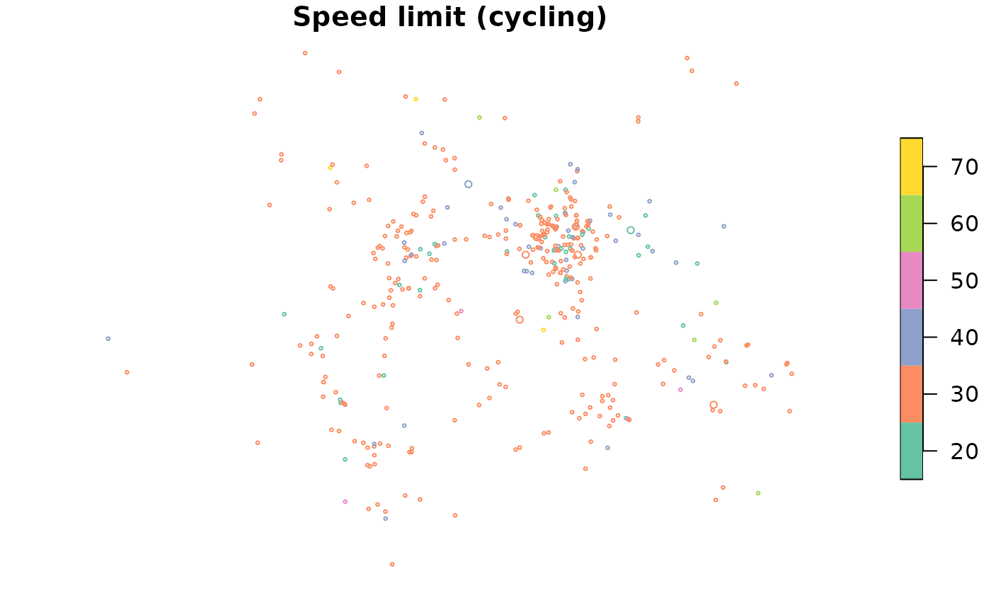
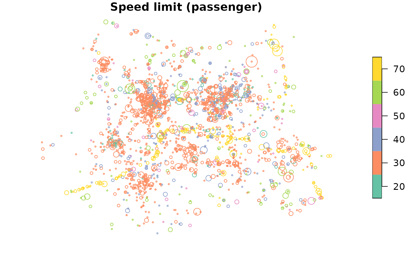
The spatial distribution of crashes in West Yorkshire clearly relates to the region’s geography. Car crashes tend to happen on fast roads, including busy Motorway roads, displayed in yellow above. Cycling is as an urban activity, and the most bike crashes can be found in near Leeds city centre, which has a comparatively high level of cycling (compared with the low baseline of 3%). This can be seen by comparing the previous map with an overview of the area, from an academic paper on the social, spatial and temporal distribution of bike crashes (Lovelace, Roberts, and Kellar 2016):
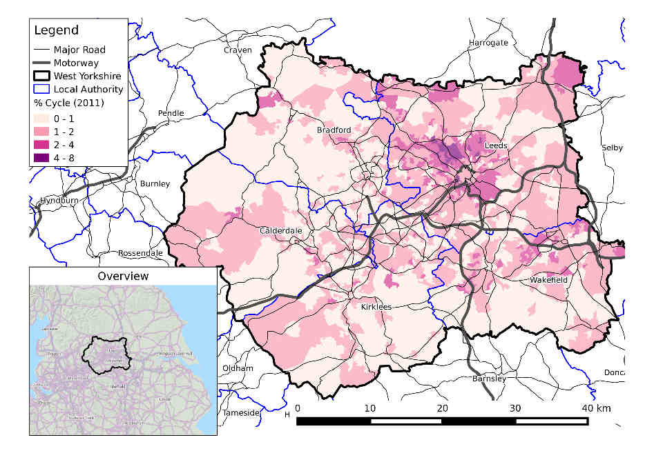
In addition to the Total number of people hurt/killed,
cj contains a column for each type of casualty (cyclist,
car occupant, etc.), and a number corresponding to the number of each
type hurt in each crash. It also contains the geometry
column from crashes_sf. In other words, joins allow the
casualties and vehicles tables to be geo-referenced. We can then explore
the spatial distribution of different casualty types. The following
figure, for example, shows the spatial distribution of pedestrians and
car passengers hurt in car crashes across West Yorkshire in 2022:
library(ggplot2)
crashes_types = cj %>%
  filter(collision_severity != "Slight") %>%
  mutate(type = case_when(
    walking > 0 ~ "Walking",
    cycling > 0 ~ "Cycling",
    passenger > 0 ~ "Passenger",
    TRUE ~ "Other"
  ))
crashes_types$speed_limit = as.integer(crashes_types$speed_limit)
table(crashes_types$speed_limit)
#>
#>  20  30  40  50  60  70
#> 100 848 155  30  75  63
ggplot(crashes_types, aes(size = Total, colour = speed_limit)) +
  geom_sf(show.legend = "point", alpha = 0.3) +
  facet_grid(vars(type), vars(collision_severity)) +
  scale_size(
    breaks = c(1:3, 12),
    labels = c(1:2, "3+", 12)
    ) +
  scale_color_gradientn(colours = c("blue", "yellow", "red")) +
  theme(axis.text = element_blank(), axis.ticks = element_blank())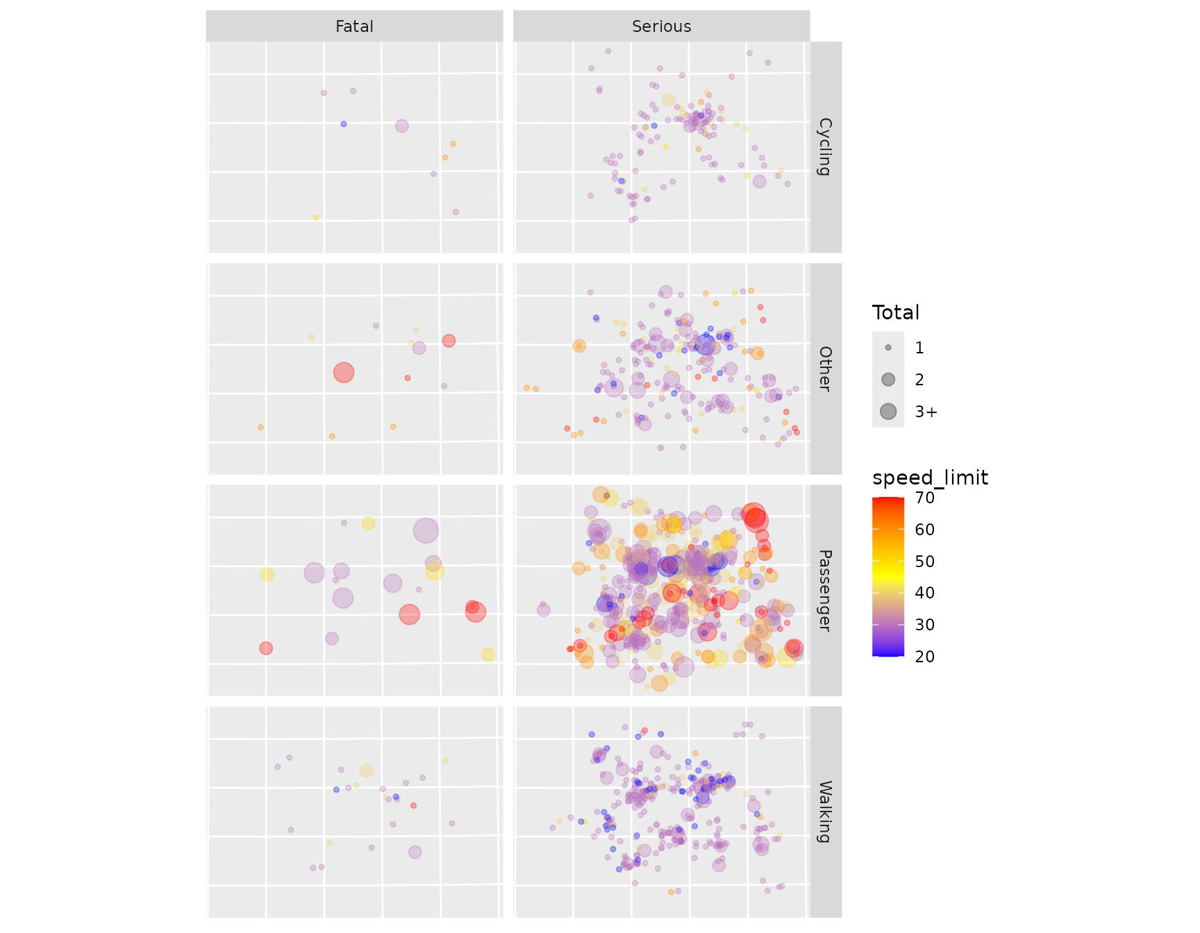
Spatial distribution of serious and fatal crashes in West Yorkshire, for cycling, walking, being a car passenger and other modes of travel. Colour is related to the speed limit where the crash happened (red is faster) and size is proportional to the total number of people hurt in each crash (legend not shown).
It is clear that different types of road users tend to get hurt in different places. Car occupant casualties (labelled ‘passengers’ in the map above), for example, are comparatively common on the outskirts of cities such as Leeds, where speed limits tend to be higher and where there are comparatively higher volumes of motor traffic. Casualties to people on foot tend to happen in the city centres. That is not to say that cities centres are more dangerous per unit distance (typically casualties per billion kilometres, bkm, is the unit used) walked: there is more walking in city centres (you need a denominator to estimate risk).
To drill down further, we can find the spatial distribution of all pedestrian casualties, broken-down by seriousness of casualty, and light conditions. This can be done with tidyvers functions follows:
table(cj$light_conditions)
#>
#> Darkness - lighting unknown       Darkness - lights lit
#>                          81                        1136
#>     Darkness - lights unlit      Darkness - no lighting
#>                          40                         117
#>                    Daylight
#>                        3026
cj$speed_limit = as.integer(cj$speed_limit)
cj %>%
  filter(walking > 0) %>%
  mutate(light = case_when(
    light_conditions == "Daylight" ~ "Daylight",
    light_conditions == "Darkness - lights lit" ~ "Lit",
    TRUE ~ "Other/Unlit"
  )) %>%
  ggplot(aes(colour = speed_limit)) +
  geom_sf() +
  facet_grid(vars(light), vars(collision_severity)) +
  scale_color_continuous(low = "blue", high = "red") +
  theme(axis.text = element_blank(), axis.ticks = element_blank())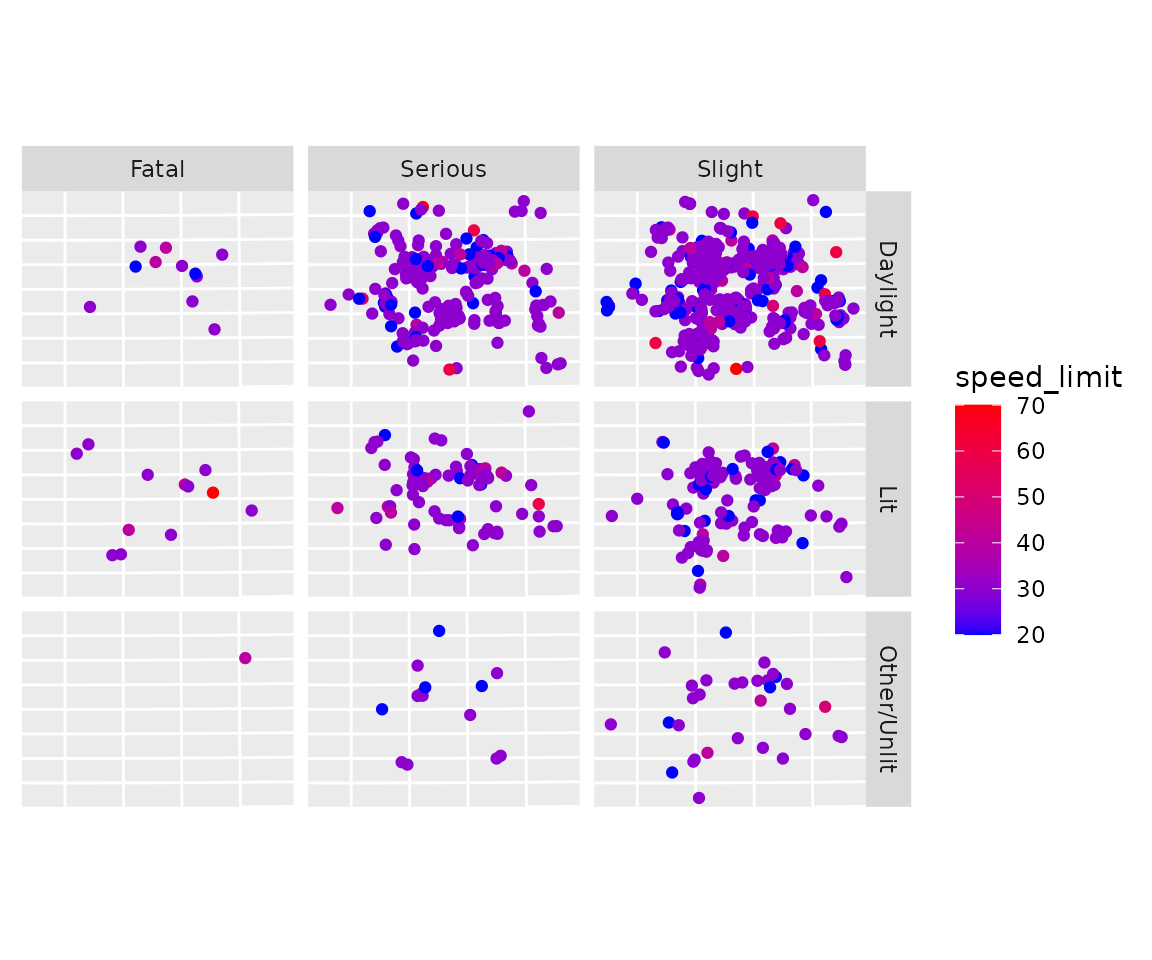
Time series analysis
We can also explore seasonal and daily trends in crashes by aggregating crashes by day of the year:
crashes_dates = cj %>%
  st_set_geometry(NULL) %>%
  group_by(date) %>%
  summarise(
    walking = sum(walking),
    cycling = sum(cycling),
    passenger = sum(passenger)
    ) %>%
  gather(mode, casualties, -date)
ggplot(crashes_dates, aes(date, casualties)) +
  geom_smooth(aes(colour = mode), method = "loess") +
  ylab("Casualties per day")
#> `geom_smooth()` using formula = 'y ~ x'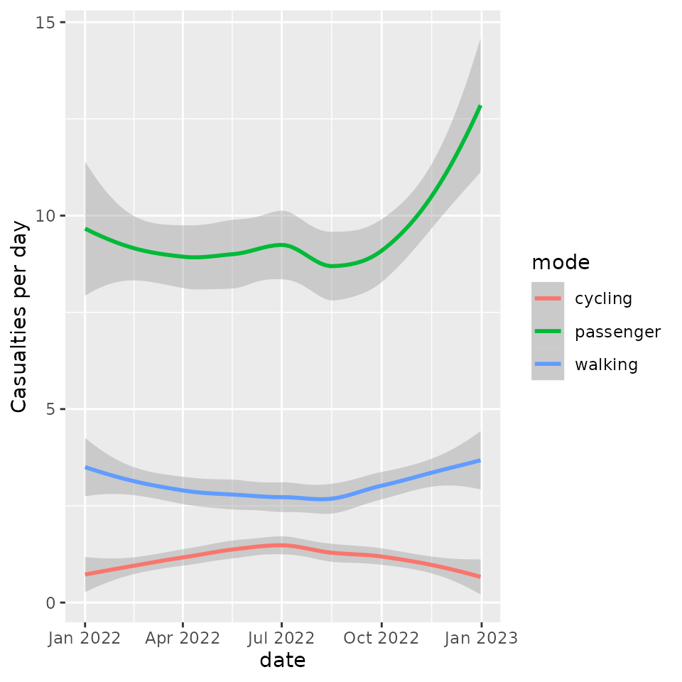
Different types of crashes also tend to happen at different times of day. This is illustrated in the plot below, which shows the times of day when people who were travelling by different modes were most commonly injured.
library(stringr)

crash_times = cj %>%
  st_set_geometry(NULL) %>%
  group_by(hour = as.numeric(str_sub(time, 1, 2))) %>%
  summarise(
    walking = sum(walking),
    cycling = sum(cycling),
    passenger = sum(passenger)
    ) %>%
  gather(mode, casualties, -hour)

ggplot(crash_times, aes(hour, casualties)) +
  geom_line(aes(colour = mode))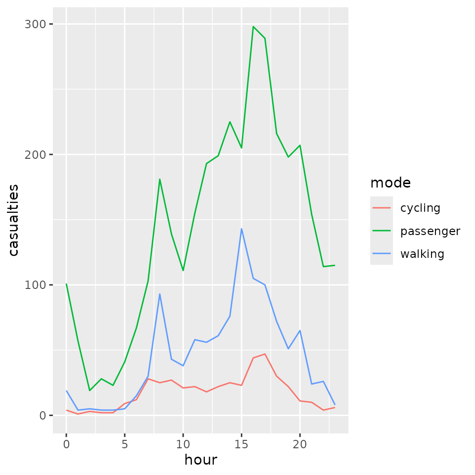
Note that bike crashes tend to have distinct morning and afternoon peaks, in-line with previous research (Lovelace, Roberts, and Kellar 2016). A disproportionate number of car crashes appear to happen in the afternoon.
Further work
There is much potential to extend the package beyond downloading, reading and formatting STATS19 data. The greatest potential is to provide functions that will help with analysis of STATS19 data, to help with road safety research. Much academic research has been done using the data, a few examples of which are highlighted below to demonstrate the wide potential for further work.
- Research exploring the effectiveness of road safety policies such as speed limits. An example in this area is this paper on 20 mph zones who found that areas with 20mph speed limits were safer. This raises the question: can the same result be repeated using reproducible methods? Does the finding hold for more recent 20 mph zones? Is the recent finding of the Department for Transport’s (2018) research, that 20 mph zones alone do not reduce crash rates, supported by reproducible analysis? What are the factors that make speed limits more or less effective (see sarkar_street_2018? for example)?
- Research into weather as a contributing factor to road traffic casualties (e.g. Edwards 1998). This raises the question: could matching crash data from the STATS19 data with historic weather data from other R packages help advance knowledge in this area?
- Assessment of crash rates normalised by estimated exposure rates (risk). An example of this type of research by an author of the package found substantial spatial variation in the number of cyclist casualties across West Yorkshire (Lovelace, Roberts, and Kellar 2016). This raises the questions: are similar spatial differences found in other regions? What are the factors leading to relatively high and low rates of different types of crash?
The broader point is that the stats19 package could help road safety research, by making open access data on road crashes more accessible to researchers worldwide. By easing the data download and cleaning stages of research, it could also encourage reproducible analysis in the field.
There is great potential to add value to and gain insight from the data by joining the datasets with open data, for example from the Consumer Data Research Centre (CDRC, which funded this research), OpenStreetMap and the UK’s Ordnance Survey. If you have any suggestions on priorities for these future directions of (hopefully safe) travel, please get in touch on at github.com/ITSLeeds/stats19/issues.