Route networks with stplanr

library(stplanr)
library(sf)

Introduction

Route networks represent the network of highways, cycleways, footways and other ways along which transport happens. You can get route network data from OpenStreetMap (e.g. via the osmdata R package) and other providers or transport network data.

Creating route networks from overlapping routes

Unlike routes, each segment geometry in a route network can only appear once.

stplanr can be used to convert a series of routes into a route network, using the function overline(), as illustrated below:

library(stplanr)
library(sf)
sample_routes <- routes_fast_sf[2:6, 1]
sample_routes$value <- rep(1:3, length.out = 5)
rnet <- overline(sample_routes, attrib = "value")
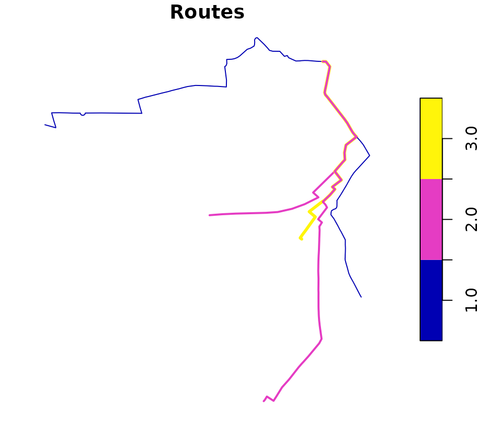
plot(sample_routes["value"], lwd = sample_routes$value, main = "Routes")
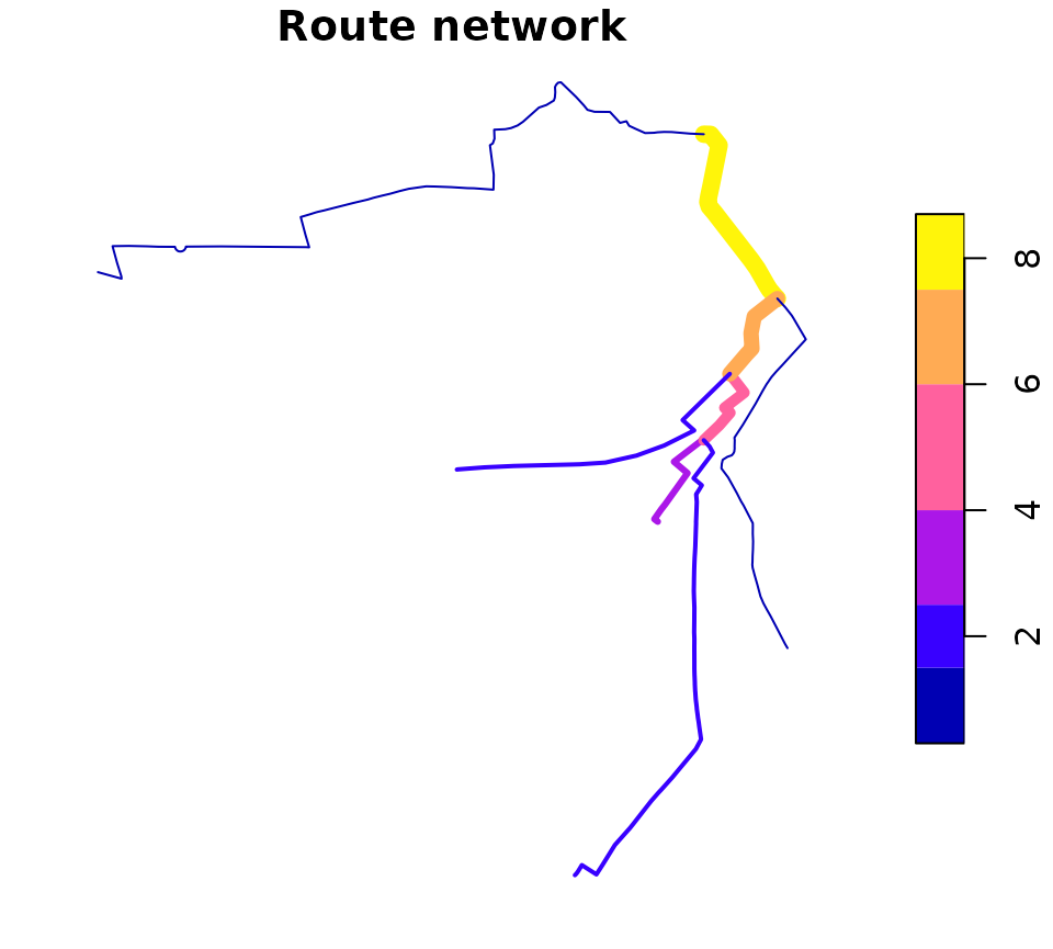
plot(rnet["value"], lwd = rnet$value, main = "Route network")

The above figure shows how overline() breaks the routes into segments with the same values and removes overlapping segments. It is a form of geographic aggregation.

Identifying route network groups

Route networks can be represented as a graph. Usually all segments are connected together, meaning the graph is connected. We can show that very simple network above is connected as follows:

touching_list = st_intersects(sample_routes)
g = igraph::graph.adjlist(touching_list)
#> Warning: `graph.adjlist()` was deprecated in igraph 2.0.0.
#> ℹ Please use `graph_from_adj_list()` instead.
#> This warning is displayed once every 8 hours.
#> Call `lifecycle::last_lifecycle_warnings()` to see where this warning was
#> generated.
igraph::is_connected(g)
#> [1] TRUE

A more complex network may not be connected in this way, as shown in the example below:

# piggyback::pb_download_url("r_key_roads_test.Rds")
u = "https://github.com/ropensci/stplanr/releases/download/0.6.0/r_key_roads_test.Rds"
rnet_disconnected = readRDS(url(u))
touching_list = sf::st_intersects(rnet_disconnected)
g = igraph::graph.adjlist(touching_list)
igraph::is_connected(g)
#> [1] FALSE
sf:::plot.sfc_LINESTRING(rnet_disconnected$geometry)

The elements of the network are clearly divided into groups. We can identify these groups as follows:

rnet_disconnected$group = rnet_igroup(rnet_disconnected)

Routing on route networks

# plot(rnet$geometry)
# plot(sln_nodes, add = TRUE)
# xy_path <- sum_network_routes(sln = sln, start = xy_nodes[1], end = xy_nodes[2], sumvars = "length")
# # xy_path = sum_network_links(sln = sln, start = xy_nodes[1], end = xy_nodes[2])
# plot(rnet$geometry)
# plot(xy_sf$geometry, add = TRUE)
# plot(xy_path$geometry, add = TRUE, lwd = 5)

Adding new nodes

New nodes can be added to the network, although this should be done before the graph representation is created. Imagine we want to create a point half way along the the most westerly route segment in the network, near the coordinates -1.540, 53.826:

new_point_coordinates <- c(-1.540, 53.826)
p <- sf::st_sf(geometry = sf::st_sfc(sf::st_point(new_point_coordinates)), crs = 4326)

Other approaches

Other approaches to working with route networks include:

• sDNA, an open source C++ library for analysing route networks and estimating flows at segments across network segments
• sfnetworks, an R package that provides an alternative igraph/sf spatial network class
• dodgr, an R package providing functions for calculating distances on directed graphs
• cppRouting, a package for routing in C++
• Chapter 10 of Geocomputation with R, which provides context and demonstrates a transport planning workflow in R.